It's a topic we touch upon from time to time as it relates to things like how stock prices behave or how the economy works, but emergence is much more than that. Quanta Magazine's short 3-and-a-half-minute video from their In Theory series provides a taste of what it is and where else it is seen:

Quanta's John Rennie explains the wonderful way complex order comes into being:

Nature is filled with such examples of complex behaviors that arise spontaneously from relatively simple elements. Researchers have even coined the term “emergence” to describe these puzzling manifestations of self-organization, which can seem, at first blush, inexplicable. Where does the extra injection of complex order suddenly come from?

Answers are starting to come into view. One is that these emergent phenomena can be understood only as collective behaviors — there is no way to make sense of them without looking at dozens, hundreds, thousands or more of the contributing elements en masse. These wholes are indeed greater than the sums of their parts.

Another is that even when the elements continue to follow the same rules of individual behavior, external considerations can change the collective outcome of their actions. For instance, ice doesn’t form at zero degrees Celsius because the water molecules suddenly become stickier to one another. Rather, the average kinetic energy of the molecules drops low enough for the repulsive and attractive forces among them to fall into a new, more springy balance. That liquid-to-solid transition is such a useful comparison for scientists studying emergence that they often characterize emergent phenomena as phase changes.

If you have a spare hour and 13 minutes, you can hear economists Don Boudreaux, Mike Munger, and Russ Roberts discuss how emergent orders arise in human activities via an EconTalk podcast!

The Navier-Stokes equations describing the flow of fluids are among the most useful math equations that have ever been developed. So much so that if a mathematician should someday demonstrate they can either demonstrate the equations will always work or can provide an example where they do not, they will win a $1 million prize from the Clay Mathematics Institute for solving one of its Millennium Problems.

In doing that, the eventual winner of the prize will be able to predictably explain how order, in the form of the smooth, laminar flow of an incompressible (contant density) fluid, transitions into disorderly turbulence, as illustrated in the following mesmerizing two-and-a-half minute video from the Lutetium Project:

And they will be also be able to accurately describe how some sense of order might spontaneously emerge from turbulent flow, as recently modeled for a recent paper using the Navier-Stokes equations by Florian Reetz, Tobias Kreilos and Tobias M. Schneider of the Ecole polytechnique fédérale de Lausanne (EPFL). The following image from EPFL shows the emergence of an orderly, layered structure within a turbulent flow from their modeling work.

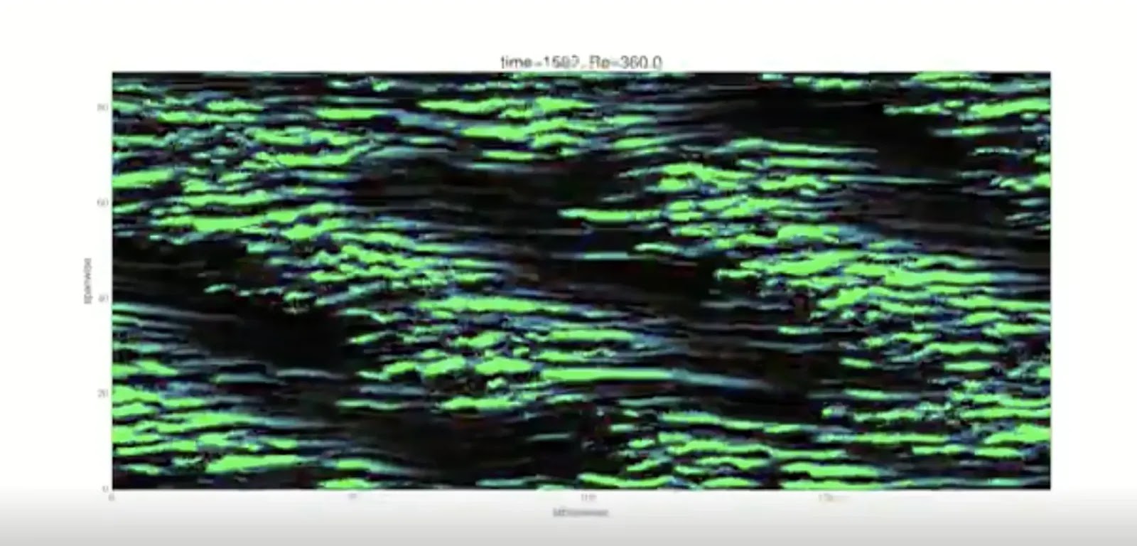
Here's why the application of Navier-Stokes equations to reveal this pattern is such a big deal:

Though physicists had observed this phenomenon experimentally, they can now explain why this happens using fundamental fluid dynamics equations, bringing them a step closer to understanding why particles behave in this way. [The Biggest Unsolved Mysteries in Physics]

In the lab, when a fluid is placed in between two parallel plates that are moving in opposite directions from each other, its flow becomes turbulent. But after a little while, the turbulence starts to smooth out in a striped pattern. What results is a canvas of smooth and turbulent lines running at an angle to the flow (imagine slight wind-created waves in a river).

"You get structure and clear order out of the chaotic motion of turbulence," said senior author Tobias Schneider, an assistant professor in the school of engineering at the Swiss Federal Institute of Technology Lausanne. This "kind of weird and very obscure" behavior has "fascinated scientists for a long, long time."

Physicist Richard Feynman predicted that the explanation must be hidden in fundamental equations of fluid dynamics, called the Navier-Stokes equations.

But these equations are very difficult to solve and analyze, Schneider told Live Science. (Showing that the Navier-Stokes equations even have a smooth solution at every point for a 3D fluid is one of the $1 million Millennium Prize problems.) So up until this point, no one knew how the equations predicted this pattern-forming behaviors. Schneider and his team used a combination of methods, including computer simulations and theoretical calculations to find a set of "very special solutions" to these equations that mathematically describe each step of the transition from chaos to order.

While not the kind of mathematical proof that will win the million-dollar Millennium Prize, Reetz, Kreilos and Schneider have created a remarkable demonstration of the ability of Navier-Stokes equations to accurately describe some of the chaotic mechanics of fluids in motion that are observed in the real world.

As for the status of the Navier-Stokes Millennium Prize, the jury is still out on whether Tristan Buckmaster and Vlad Vicol's initial work demonstrating that the equations do not always generate unique solutions will claim the prize, which we have previously described as the biggest math story of 2017. They have since teamed with Maria Colombo on a new paper (preprint available via arXiv) in following up the topic.

References

Florian Reetz, Tobias Kreilos & Tobias M. Schneider. Exact invariant solution reveals the origin of self-organized oblique turbulent-laminar stripes. Nature Communications 10, 2277 (2019). DOI: 10.1038/s41467-019-10208-x. 23 May 2019.

The Lutetium Project. The transition to turbulence. [Online Video]. 15 November 2016.

Image Credits via Creative Commons Attribution 4.0 International License.

If you've ever had to deal with a pair of earphones after they've become tangled, you know exactly what kind of mess they can make and what kind of pain they can be to untangle. Is there anything you can do about it?

Before we go any further, let's draw some lessons from science for how cords can almost spontaneously become tangled from the following video:

Now, let's get to the practical matter of finding out how likely your cords will become tangled. In the following tool, we've adapted the math developed by Dorian M. Raymer and Douglas E. Smith in their 2007 paper to calculate the probability that your cord/string/rope will become tangled, assuming that it is made of a medium-stiffness material, based upon its length. If you're reading this article on a site that republishes our RSS news feed, click here to access a working version of this tool!

If your cord has a relatively low probability of becoming knotted or tangled, say below 5 or 10%, you might not need to worry much about taking any special measures to keep it that way.

But, if you want to avoid the hassles that come from your cords becoming tangled, you might consider the suggestions from the video, using shorter, stiffer cords (if feasible) or getting smaller containers to store your longer cords (if not).

Meanwhile, if you're looking to learn more about knot theory, and yes, there is such a thing in maths, here's a quick introduction:

References

Raymer, Dorian M. and Smith, Douglas E. Spontaneous knotting of an agitated string. PNAS. October 16, 2007 104 (42) 16432-16437; https://doi.org/10.1073/pnas.0611320104. Note: For our tool, we corrected the L₀ parameter to be 1.025 after replicating the other parts of the authors' logistic function regression using the data presented in Figure 2, where our L₀ correction allowed us to replicate their reported probabilities for various cord lengths.

On 24 September 2018, mathematician Michael Atiyah announced that he believed that he had cracked the Riemann Hypothesis at the Heidelberg Laureate Forum, which if his proof holds, would represent a very big deal. Not just because the proof would come with a one million dollar prize from solving one of the Clay Mathematical Institute's millennium problems, or because it describes the distribution of prime numbers, but also because it would automatically prove a lot of other mathematical hypotheses that rely on the Riemann hypothesis being valid for their contentions to hold.

For more information about what the Riemann Hypothesis is, we recommend viewing either Numberphile's 17-minute video or 3Blue1Brown's 22-minute long video on the topic, both of which are well done but offer different strengths in presentation. What we found interesting in Atiyah's announcement is that he claims the proof came about because of work he was doing (leaked here?) to analytically derive the fine structure constant from physics, which is fascinating in and of itself.

In the following video from the University of Nottingham's Sixty Symbols project, Laurence Eaves provides a blissfully short 5-minute long explanation of the significance of the fine structure constant, which is the measure of the strength of the electromagnetic force governing how electrically-charged elementary particles interact.

The three fundamental constants that are combined in the fine structure constant are:

• The elementary charge of an electron (e)
• Planck's constant, divided by both 2 and pi (h)
• The speed of light (c)

If we include pi, there are technically four universal constants in the formulation. It's estimated to be very nearly equal to 1 divided by 137, where if it were exactly equal to that ratio, would really be extraordinary because the value 137 happens to also be a Pythagorean prime number. As it happens, the denominator in the fine structure constant is currently estimated to be 137.035999138..., so it's close, but not quite.

Did you ever want to get into quantum physics, but didn't know where to start?

A good place to begin understanding a complex, complicated thing like quantum mechanics is at the beginning, where believe it or not, it all started with, dare we say, a light bulb moment! Check out the following video from MinutePhysics on the origin of quantum mechanics, which is really all about how physics works on the tiniest scales possible.

If you're ready to move on to the next level, you might enjoy Dominic Walliman's explanation of Quantum Physics for 7 Year Olds. After that, before you get cocky, remember that "nobody understands quantum mechanics!"

Previously, we established that there is a rather strong correlation between changes in the acceleration of nominal private sector debt in the U.S. and the direction of growth for the nation's real GDP growth rate. In a nutshell, we found that "nearly 88% of periods in which the trailing twelve month average of private debt acceleration declined or was negative occurred when the U.S.' real GDP growth rate was falling", indicating that changes in the acceleration of private debt is a good predictor of the direction of GDP growth.

Why such a strong correlation between nominal private debt and real GDP? Unlike money borrowed by government entities, when people or businesses take out loans in the private sector of the economy, they do so only when they can reasonably anticipate that they will be able to generate the income or revenue needed to pay their creditors back over the terms of their loans. If they anticipate that they will have a hard time doing that going forward, they will avoid taking on debt, and vice versa - they will increase the rate of their borrowing if they anticipate having an easier time paying it back.

With the Federal Reserve having released its flow of funds data through the end of the third quarter of 2015 in the past week, we can now introduce our chart showing our calculated acceleration rate for private sector debt in the U.S. and its trailing year average against the backdrop of periods of falling GDP growth rates, recessions and the Federal Reserve's various Quantitative Easing (QE) programs in the period from Janaury 2006 through September 2015.

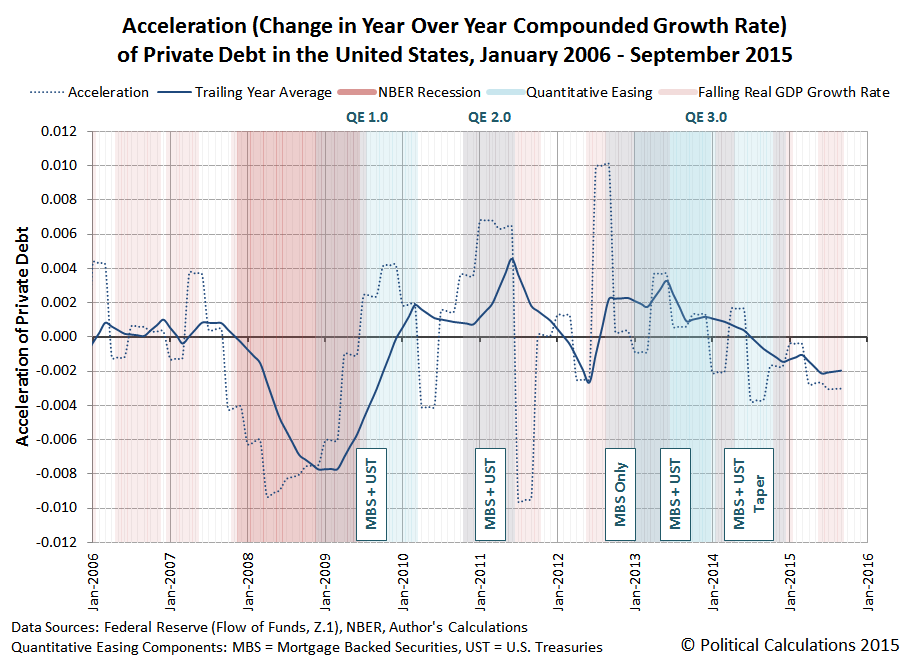
We see that in the third quarter of 2015, the acceleration of private debt in the U.S. remained negative, declining slightly from the previous quarter. Correspondingly, the BEA's second estimate of real GDP for the quarter indicates that its growth rate is likewise falling.

One thing to keep in mind when considering this information is that the U.S. Bureau of Economic Analysis can make significant revisions to its estimates of the nation's GDP during the first several years after it releases its initial estimates as it acquires more accurate and detailed information about the level of economic activity.

For example, the BEA's first estimate for GDP in the third quarter of 2012, released on 26 October 2012 just ahead of the last U.S. presidential elections, indicated that the real GDP growth rate for the quarter was +2.0%, up from the preceding quarter's real growth rate of +1.3%.

But now, according to Table 1 of the BEA's second estimate of GDP for the third quarter of 2015, which was released on 24 November 2015, we find that the real GDP growth rate of 2012-Q3 is now estimate to be just +0.5%, having fallen from the preceding quarter's real growth rate of +1.9%, as the economy of the U.S. was actually in the process of stalling out at that time. Only the U.S. Federal Reserve's expected intervention through its third Quantitative Easing program (QE 3.0), and its boosting effect on private debt, prevented the U.S. economy from fully sinking into recession at that time.

It will be interesting to see how the acceleration of private debt in the U.S. evolves should the Federal Reserve finally follow through on its plans to start hiking short term interest rates in the U.S. in the absence of any additional quantitative easing programs later this week.

Data Sources

U.S. Federal Reserve. Data Download Program. Z.1 Statistical Release (Total Liabilities for All Sectors, Rest of the World, State and Local Governments Excluding Employee Retirement Funds, Federal Government). 1951Q4 - 2015Q3. [Excel Spreadsheet]. Online Database. 10 December 2015. Accessed 14 December 2015.

U.S. Bureau of Economic Analysis. Table 1.1.1. Percent Change from Preceding Period in Real Gross Domestic Product.
1947Q1 through 2015Q3 (second estimate). Online Database]. Accessed 14 December 2015.

References

National Bureau of Economic Research. U.S. Business Cycle Expansions and Contractions. [PDF Document]. Accessed 14 December 2015.

da Costa, Polyana and Ponder, Crissinda. How Fed Moves Affect Mortgage Rates. (Timeline for Federal Reserve Quantitative Easing Programs QE 1.0 through 3.0). [Online Article]. 17 September 2015. Accessed 14 December 2015.

Previously on Political Calculations

Political Calculations. The Position, Velocity and Accelration of Private Debt in the U.S.. 5 November 2015.

Political Calculations. The Correlation Between Decelerating Debt and Falling GDP. 12 November 2015.

Political Calculations. QE and the Acceleration of Private Debt in the U.S.. 18 November 2015.

What effect has the Federal Reserve's previous Quantitative Easing (QE) programs had on the acceleration of private debt in the U.S. economy?

That's an important question to answer because of the remarkable correlation between the nation's real economic growth rate and the change in the rate of growth of private debt in the U.S., where periods of a rising real GDP growth rate are associated with a rising acceleration of private debt, and periods of falling real GDP growth are correlated with decelerating private debt.

In the chart below, we've visualized the periods in which the Fed's three major QE programs of recent years provide the backdrop against the trajectory of the acceleration of private debt and its trailing twelve month average. For reference, we've also indicated the period of the so-called "Great Recession", as determined by the National Bureau of Economic Research.

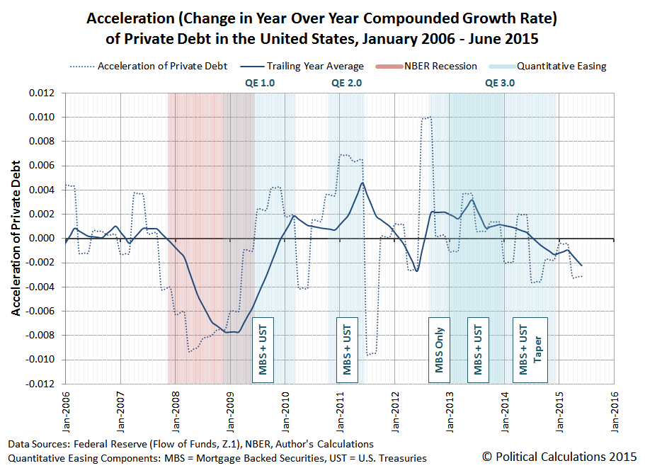
In the chart above, we've also identified the kinds of assets that the Federal Reserve's focused on purchasing during each of the major phases of its QE programs, Mortgage Backed Securites (MBS) and U.S. Treasuries (UST).

What we observe in the trailing year data is that the Fed's various QE programs have had a fairly clear "on-off" effect on changes in the rate of growth of private debt in the U.S. economy, which is especially evident for QE 1.0 and QE 2.0., with the acceleration of private debt being jerked upward coincidentally or soon after when the Fed's QE programs were turned "on", and jerked downward almost instantly when the applied impulse of QE was turned "off".

The results for QE 3.0 are different in that the Fed's asset buying programs were structured differently from its previous programs. Here, the acceleration of private debt received an immediate upward jerk as the Fed initially began only purchasing MBS assets, but when the Fed expanded its third QE program in January 2013 to include U.S. Treasuries, the upward jerk would appear to be somewhat delayed.

We suspect that apparent delay is due to the then-looming impact of the U.S. government's fiscal cliff crisis, which was prompted by the re-election of President Obama and the expectation that the very large tax hikes that he favored would into effect on 1 January 2013 as a consequence, which weighed down the acceleration of private debt going into the end of 2012.

The Fed, seeing the economic drag from those expectations, announced in December 2012 that it would expand its third QE program in Janaury 2013 to include U.S. Treasuries, which would compensate for the negative effects of those tax hikes on the weakened U.S. economy of late 2012. (The 2012 fiscal cliff crisis was resolved on 3 January 2013 with a compromise that raised tax rates, but to a lesser extent than would have otherwise, but not before the damage to the acceleration of private debt was done.)

After 2013, the Fed began steadily tapering its purchases of UST and MBS assets, which coincides with a generally decreasing acceleration for private debt in the U.S. economy, which has continued to fall fairly steadily since. Since August 2014, the level of acceleration of private debt in the U.S. has also been negative. Through June 2015, the trailing year average of private debt acceleration in the U.S. has not yet reached the levels where the Fed has launched its previous rounds of quantitative easing in its attempts to stimulate the debt-funded growth of the U.S. economy.

On a final side note, in previous posts, we've described the Fed's addition of U.S. Treasuries to its its third QE asset purchase program as QE 4.0, although in retrospect, it's really better understood as an expansion of QE 3.0. If you happen to come across older posts of ours (before 18 November 2015) where we reference QE 4.0, that's what we're referring to! Any reference of ours to QE 4.0 after 18 November 2015 would be with respect to a new QE program, which we would see as becoming more and more likely with the continued deceleration of the growth of private debt in the U.S. economy....

Data Sources

U.S. Federal Reserve. Data Download Program. Z.1 Statistical Release (Total Liabilities for All Sectors, Rest of the World, State and Local Governments Excluding Employee Retirement Funds, Federal Government). 1951Q4 - 2015Q2. [Online Database]. 18 September 2015. Accessed 28 October 2015.

National Bureau of Economic Research. U.S. Business Cycle Expansions and Contractions. [PDF Document]. Accessed 28 October 2015.

As promised, today we're doing something more interesting with the Federal Reserve's data for the level of private debt that has accumulated over time in the United States than just calculating its amount, it year over year rate of growth (or velocity) and also the rate of change in its year over year growth rate (or acceleration).

Starting with our results for the acceleration for private debt, we first calculated its trailing twelve month average to smooth out the volatility in our results to better capture its general trends during the period from January 1955 through June 2015.

We next extracted the U.S. Bureau of Economic Analysis' data on the quarterly growth rate of real (inflation-adjusted) Gross Domestic Product (GDP) spanning the same period, using linear interpolation to estimate the real growth rate in the months in between the months ending each calendar quarter, and then calculating the trailing twelve month average of the real GDP growth rate to smooth out the volatility in the results and to better capture the general trends in real GDP growth rates over time.

We then graphed both the acceleration of private debt (dotted blue line) and its trailing twelve month average (solid blue line) in the chart below, in which we've also indicated the periods for when the real growth rate of U.S. GDP was falling (shown as the light red vertical bands). For added measure, we've also indicated the periods in which the National Bureau of Economic Research has determined the U.S. economy was in recession (darker red vertical bands).

What we observe in the chart above is a really remarkable correlation. When the general rate of acceleration of private debt in the U.S. is falling, very much more often than not, such periods either precede or coincide with the periods in which the real rate of growth of the U.S. economy was also falling.

We next calculated some very basic statistics related to that basic correlation. In the 726 months from January 1955 through June 2015, we counted a total of 395 in which the trailing twelve month rate of growth of GDP in the U.S. was falling and a total 366 in which the trailing twelve month average rate of acceleration was falling.

There were 245 months in which both the trailing twelve month averages of both the acceleration of private debt and the growth rate of real GDP in the U.S. were both falling. That works out to be a correlation of nearly 65% for periods in which the trailing twelve month average of private debt acceleration declined, or 62% if we look just at the periods in which the trailing twelve month average of the real GDP growth rate declined.

That works out to be very close to the results that Michael Biggs, Thomas Mayer and Andreas Pick found in their 2010 paper, in which they worked out the correlation between changes in the acceleration of debt and the level of employment in the U.S, which Steve Keen summarized that year (emphasis ours):

They first showed the cor­re­la­tion between what they called “the credit impulse”—the rate of change of the rate of change of debt, divided by GDP—and both GDP and employ­ment (for those who have access to research from Deutsche Secu­ri­ties, they have a sim­pler expla­na­tion of their analy­sis in Global Macro Issues for Decem­ber 17 2009: “The myth of the credit-less recovery”).

The chart below shows my con­fir­ma­tion of the rela­tion­ship with the data on the annual change in unem­ploy­ment in the USA and the annual rate of accel­er­a­tion of pri­vate debt since 1955. The cor­re­la­tion is –0.67: a stag­ger­ing cor­re­la­tion of a first and a sec­ond order vari­able over such a period, and across both booms and busts.

We noted above that the change in the rate of acceleration of private debt often either leads or coincides with changes in the real GDP growth rate, which is something that we can directly observe in the acceleration of private debt in the U.S. turning downward before as as the real GDP growth rate in the U.S. falls, and also as it turns upward either before or as the real GDP growth rate in the U.S. rises, which is very clearly evident during the periods in which the U.S. economy was in recession.

It occurred to us that the simple correlation between a declining rate of acceleration for private debt and a falling rate of real GDP growth isn't necessarily capturing the full dynamic between the two. So we went the extra mile and calculated the correlation for when the trailing twelve month average of private debt acceleration was either falling or negative and the periods in which the real growth rate of U.S. GDP was falling.

For the period from January 1955 through June 2015, we found that nearly 88% of periods in which the trailing twelve month average of private debt acceleration declined or was negative occurred when the U.S.' real GDP growth rate was falling, and if we look just at the periods in which the trailing twelve month average of the real GDP growth rate declined, we find that nearly 84% of those periods are ones in which the acceleration of private debt was either falling or negative.

Speaking of which, in looking at the period since June 2013, we see that the acceleration of private debt in the U.S. has been falling and, through June 2015, the most recent month for which we have data, has become negative. We expect that the U.S. Federal Reserve will update its data for the U.S.' private debt through September 2015 sometime in mid-December 2015.

Update 14 December 2015: Added the words "growth rate" in boldface type to the second to last paragraph above for clarification.

References

Political Calculations. The Position, Velocity and Acceleration of Private Debt. [Online Article]. 5 November 2015.

Biggs, Michael and Mayer, Thomas and Pick, Andreas, Credit and Economic Recovery: Demystifying Phoenix Miracles (March 15, 2010). Available at SSRN: http://ssrn.com/abstract=1595980 or http://dx.doi.org/10.2139/ssrn.1595980.

Keen, Steve. Deleveraging, Deceleration and the Double Dip. Steve Keen's Debtwatch. [Online article]. 10 October 2010. Accessed 28 October 2015.

Data Sources

U.S. Federal Reserve. Data Download Program. Z.1 Statistical Release (Total Liabilities for All Sectors, Rest of the World, State and Local Governments Excluding Employee Retirement Funds, Federal Government). 1951Q4 - 2015Q2. [Online Database]. 18 September 2015. Accessed 28 October 2015.

U.S. Bureau of Economic Analysis. National Income and Product Accounts. Table 1.1.1. Percent Change from Preceding Period in Real Gross Domestic Product. 1947Q1 through 2015Q3 (first estimate). [Online Database]. Accessed 28 October 2015.

National Bureau of Economic Research. U.S. Business Cycle Expansions and Contractions. [PDF Document]. Accessed 28 October 2015.

Now that stock prices are once again reaching near the levels where they peaked before they crashed back on 20 August 2015, a lot of people are wondering if the U.S. stock market has gotten back to normal.

That supposes that anyone has some idea of what normal might look like for stock prices. As it happens, we do, provided that we define "normal" as being consistent with the trend in U.S. stock prices with respect to their trailing year dividends per share that existed prior to order breaking down in the stock market, because we could at least use the tools of statistical analysis to describe the variation of stock prices about that trend.

So here you go....

What we find is that given the level of trailing year dividends per share that we're on track to hit in the fourth quarter of 2015, the value of the S&P 500 would have to be over 150 points higher than it is now to be considered to be back on that track.

Of course, we should acknowledge that the variation in stock prices really isn't well described by a Gaussian, or "normal" distribution. The variation with respect to the central trend is really a lot more consistent with the kind of Lévy distribution that goes along with stock prices traveling a quantum random walk.

Rather like the blue-dashed bell curve shown in the diagram comparing the Lévy distribution with Cauchy and Gaussian "normal" bell curves below, as extracted from Greg Randall's lectures at MIT back in 2003:

But the bottom line is that stock prices are not "back to normal". Mainly because they're not really normal to begin with!

In the charts below, we're going to explore the evolution of private debt in the United States, as reported by the U.S. Federal Reserve in its Flow of Funds data, spanning all the years for which we have quarterly data, showing the results since January 1954.

Here, we've calculated private debt as the total liabilities for all sectors of the U.S. economy, less the total liabilities for the Rest of the World, State and Local Governments (less employee retirement funds), and the Federal Government.

The result of that math at the end of each calendar quarter indicates the total level of private debt in the U.S., which is equivalent to "Position" in a simple kinematics problem from high school physics. We then took those results and used linear interpolation to estimate the position of private debt for the months in between the months ending calendar quarters.

We next calculated the year over year compound rate of growth of the amount of private debt for each calendar month, which might also be described as the non-dimensionalized "Velocity" of private debt.

We then went one step further to calculate the "Acceleration" of private debt in the U.S., or rather, the change in the year over year growth rate of private debt from one month to the next.

The results of all this math are graphically presented in the three charts below, which we've lined up just like the position-velocity-acceleration versus time charts we had to draw back when we were taking basic physics!

We'll be doing something more interesting with this data soon, but in the mean time, we should recognize that we could have continued our journey down the kinematics path by also calculating the impulse, or rather the "jerk", which would be the change in acceleration of private debt. Or if we really wanted to show off, we could have progressively calculated the "jounce" (or "snap"), "crackle" and "pop" of private debt.

The resulting charts past acceleration however weren't very interesting!

Data Sources

U.S. Federal Reserve. Data Download Program. Z.1 Statistical Release (Total Liabilities for All Sectors, Rest of the World, State and Local Governments Excluding Employee Retirement Funds, Federal Government). 1951Q4 - 2015Q2. [Online Database]. 18 September 2015. Accessed 28 October 2015.