There are a lot of different ways to measure how deeply you might be in debt. You could count up all the individual credit accounts you have, such as your mortgage, your student loans, your car loan, and all your credit cards. You can also add up all the liabilities you've racked up on each of these.

But that doesn't necessarily tell you how much your personal cost of debt is. For that, you'll need to know how much you've borrowed for each of your credit accounts and the interest rate you are paying to have already borrowed what you have.

With that information, you can find what your personal cost of having debt is, taking into account how it is weighted among your different credit accounts. We've built the following tool to do that math for up to as many as six different credit accounts you might have open. If you're accessing this article on a site that republishes our RSS news feed, please click through to our site to access a working version of the tool.

In the tool above, if you have more debt accounts you would like to include in the calculation, take the results from the first six accounts, enter the total and weighted personal cost of debt interest rate in under "Credit Account #1", then continue to add the information for up to five more of your additional debt accounts. Repeat this process as necessary, until you're done. If it seems burdensome to do this, you may want to seriously consider reducing the number of credit accounts you have open.

Once you are done though, what can you do with this information?

Millionaire Mob describes it as one of the most important decision tools for making personal finance decisions you have available to you:

Personal cost of debt is so important. I cannot stress this enough. This is a line in the sand that helps you understand if you should pay down debt or invest. This is the best metric for debt prepayment....

For your personal cost of debt, you want to do anything in your ability to pay down the highest interest rate debt first. Lower your personal cost of debt to 4.5% or lower. At that point, you can invest everything you have.

The long-term average of the stock market is approximately 6-7% per year. With taxes, this is basically an annual return of about 4.5%. Thus, for every dollar you put into the stock market you should exceed your personal cost of debt. Keep in mind interest rates could increase or decrease, so this is somewhat relative.

If your final result for your personal cost of debt was above 4.5%, then taking steps to pay down your loans makes sense, where your biggest bang for the buck will come in paying down the credit that carries the highest interest rate.

We'll also note that Millionaire Mob is taking inflation into account in looking at the long term rate of return for an investment in the stock market. Over its history, the long term average rate of return for the S&P 500 is 9.4%, with the long term rate of inflation averaging about 3.3%, though the Federal Reserve has targeted a 2.0% inflation rate in recent years, which is how you get down to an investment return of 6% to 7% before you might pay taxes on your investment returns, which then drops to Millionaire Mob's threshold of 4.5% after taxes.

If you have the ability to invest with tax-free returns however, such as through a Roth IRA or a Roth 401(k), the weighted average personal cost of debt threshold for choosing between long term investing and paying down debt would rise to 6.0%, where you should choose to invest over paying down debt with any "extra" money you might have if your personal cost of debt is below that higher threshold.

Image Credit: Photo by Avery Evans on Unsplash.

Not long ago, we looked at foreign ownership of U.S. stocks, which raised a question from our readers: "How much of the world's stocks do U.S. investors own?"

We don't have a specific answer for that question, because the U.S. Treasury Department groups equities, such as stocks, in with debt having a term-to-maturity of one year or longer into the category of long-term securities in its data on the topic, where the question we can answer is "how much of the world's long-term securities do U.S. investors own?"

In the following interactive graphic, we show the answer recorded at the end of June for each year from 2002 through 2018. [If you're accessing this article on a site that republishes our RSS news feed, please click through to access a fully working version on our site, or click this link to see a static image of that chart.]

In the chart, we've compared apples-to-apples as best we can, showing the values of foreign long-term securities owned by U.S.-based investors against the backdrop of the value of U.S. long-term securities held by foreign interests.

Reviewing the history, we see that U.S. holdings of foreign long-term securities as a percent share of foreign holdings of U.S. long-term securities rose from 54% in 2002 to peak at 70% in 2007 before plunging to a low of 54% in 2010. Through 2018, it has recovered to 63% of the value of foreign-held U.S. long-term securities.

References

U.S. Department of the Treasury and Federal Reserve Bank of New York. Foreign Portfolio Holdings of U.S. Securities, as of June 29, 2018. [PDF Document]. 15 May 2019.

Komal Sri-Kumar is the president and founder of Sri-Kumar Global Strategies who just had a very interesting bit of analysis published by Bloomberg: The Bond Market Is Now a Giffen Good. In this piece, he makes the argument that sovereign debt, such as U.S. Treasuries, may be considered to be a Giffen good, which he explains in his opening paragraphs:

With some $13 trillion of bonds worldwide yielding less than zero percent, it would be easy to characterize fixed-income assets as nothing more than a giant bubble waiting to burst. Those who agree probably haven’t heard of the concept of a “Giffen good.”

Simply put, a Giffen good is a paradox of economics where rising prices lead to higher demand, which is in contrast to the negatively sloped demand curve that students learn in Economics 101. Named after 19th century Scottish economist Sir Robert Giffen, a Giffen good is typically an essential item that, because of its higher price, leaves less resources to purchase other items. (To be sure, many economists debate whether a Giffen good actually exists.)

In terms of the bond market, it’s important to understand that the rapid plunge in yields, especially for sovereign debt, reflects increased concern about the state of the global economy. Those concerns, in turn, only fuel demand for the safest assets even at negative yields, which pushes prices higher and yields even lower.

He goes on to identify three factors (which we've excerpted below) for why the interest rate yields of sovereign bonds and Treasuries are falling, which in the strange world of bond investing, means their prices are going up:

First, inflation rates have been low or declining in the U.S., euro zone and Japan, encouraging investors to allocate more resources to fixed-income assets despite falling yields. High rates of inflation reduce the purchasing power of bond holders, but low rates of inflation do the opposite....

Second, expectations for central bank monetary policy have been kind to bond investors. Ten-year yields have fallen below policy rates in the U.S., Germany and Japan, providing a reason – and pressure - for monetary authorities to reduce rates....

Third, the steep decline in U.S. and German risk-free yields have increased the attractiveness of lower-rated sovereign credits.

How long sovereign bonds and Treasuries might act like Giffen goods remains to be seen, but we should recognize that the conditions that bring Giffen goods into existence are typically transitory. Either those conditions will not endure, or should they persist, at some point, the rising prices that might have initially motivated investors to buy increased quantities of sovereign bonds may grow too high, with demand for sovereign debt sharply dropping off after that point as the Law of Demand reasserts itself.

No one really knows how high that price is. Nobody should want to find out the hard way.

More Reading

Frank Steindl introduced the concept of Money and Bonds as Giffen Goods back in December 1973, which is the earliest reference to the concept that we can find. It is also the only reference we can find before we began exploring the concept of Debt as a Giffen Good back in May 2009.

Since then, a few analysts have weighed in on the topic, including StatsGuy's Money as the Ultimate Giffen Good at The Baseline Scenario in December 2009, Eric Falkenstein's Treasuries a New Kind of Giffen Good at Falkenblog in August 2011, Kevin Erdmann's discussion of Bonds and Real Estate as Giffen Goods in May 2014, and our own followup More Evidence That Debt Is A Giffen Good in January 2017.

While not considering the role of either money or debt as a Giffen good, Timothy Taylor wrote about recent, strong evidence of Giffen Goods in Real Life at Conversable Economist in January 2012. Since the reputation of Giffen goods is that they are elusive, it's fascinating to see them documented whenever they appear.

And speaking of sovereign debt, we would be remiss if we didn't include Visual Capitalist's United Nations of Debt infographic showing data from 2017:

Nearly every nations' debt is bigger now. What could possibly go wrong?

Now that General Electric (NYSE: GE) has slashed its quarterly dividend by 91%, from $0.12 to $0.01 per share, which we estimate is about 50% more than what investors had already priced in to the stock, what can they expect next for the company's share price?

Based on the historic relationship that investors have set between the company's market capitalization and its aggregate forward year dividends since 12 June 2009, we would anticipate GE's share price falling to somewhere within a range of $3 to $7.

When GE's announced its future dividend cut on 30 October 2018, which will take effect with dividends to be paid in 2019, the company's stock price fell to $10.18 per share. Since then, the share price has continued to erode, where it has fallen into the single digits. In the absence of positive news, we would anticipate that erosion will continue until the share price stabilizes somewhere within our target range. That range is centered at about $45 billion of market capitalization, which corresponds with a share price of $5.14.

Alternatively, it is possible that the company's stock price could be sustained at higher levels if its new CEO, Larry Culp, was overly conservative in his action to preserve the company's cash by cutting its dividend. Given that GE's credit rating has been cut by S&P, Moody's and Fitch, we see that possibility as unlikely in the near term, where the reductions in its credit rating will mean higher borrowing costs going forward for a company that is awash in debt and which faces an SEC accounting investigation.

Data Sources

Dividend.com. General Electric Dividend Payout History. [Online Database]. Accessed 2 November 2018.

Ycharts. General Electric Market Cap. [Online Database]. Accessed 2 November 2018.

Yahoo! Finance. General Electric Company Historical Prices. [Online Database]. Accessed 2 November 2018.

The U.S. Department of Education has updated its statistics on the number of student loan defaults occurring within three years of a borrower beginning repayment. The latest data covers borrowers who began making payments on their student loans during the U.S. government's 2015 fiscal year, which ran from 1 October 2014 through 30 September 2015, who have subsequently stopped making scheduled payments for a prolonged period of time without making arrangements to either defer them or to seek relief from them during the following three years.

The following chart shows the number of student loan borrowers who have defaulted within three years after starting to make payments in each fiscal year from 2009 through 2015 according to the type of four year degree-granting institution they attended, covering proprietary (or for-profit) universities, public universities, and private (or non-profit) universities.

For student loan borrowers who attended four-year degree granting institutions and began making payments during the U.S. government's 2015 fiscal year, 531,653 went on to default on their student loan debt over the next three years. Of these, 51% attended public universities, 34% attended proprietary (or for-profit) institutions, and 15% attended private universities.

The next chart shows the percentage of student loan borrowers for each type of institution that began repaying their student loans, but went on to default on them within the following three years.

We find that although public universities account for the largest number of defaulting student loan borrowers, a larger percentage share of students who attend proprietary (or for-profit) institutions have consistently defaulted on their student loans.

The final chart reveals the average annual cost of college tuition and fees for each type of institution, which is based on data from the 2016-17 academic year, which is the closest we could get to 2015 for all three types of four year degree-granting institutions. The $9,670 value shown for public institutions applies for state residents eligible for in-state tuition rates, where the average public university tuition and fees for out-of-state residents is $24,820.

Since March 2010, when President Obama signed legislation putting the U.S. government into the student loan business, most of these defaults represent money borrowed from the U.S. government.

Today, about 90 percent of loans made to students and their families are from the federal government, which does not follow the same lending standards required of financial institutions. The federal government holds around $1.4 trillion in student loans on its books and is currently seeing a double digit delinquency and default rate.

10.3% of student loan borrowers who started making payments on their debt to the federal government in 2015 have defaulted. That figure has come down and stabilized over the last several years, but is still a double-digit problem for the demographic group with the lowest rate of unemployment in the U.S. economy. Meanwhile, many who are making payments on their student loans aren't getting very far in paying them down.

Just as alarming as the high number of defaults on federal student loans is that less than half of new borrowers are able to put a dent in their principal balance within three years of entering repayment.

Currently, the U.S. government makes it very difficult, if not nearly impossible for borrowers to have their student loan debts discharged through bankruptcy proceedings, which is pretty much what you would expect for any creditor who has the power to write the rules to benefit itself by forcing the repayment of any loan that it has either guaranteed or issued.

If it cannot be discharged in bankruptcy and the money borrowed is owed to the government, it isn't debt. It's taxes. The sooner that's fixed by transforming student loans back into debt, among other reforms, the better it will be for everyone involved.

References

U.S. Department of Education. Official Cohort Default Rates for Schools, by Institution Type. [PDF Documents: 2009-2011, 2012-2014, 2013-2015]. 26 September 2018. Accessed 13 October 2018.

College Board. Trends in Higher Education. Average Published Undergraduate Charges by Sector and by Carnegie Classification, 2017-18. [Online Document. 17 November 2017.

There is a rather strong correlation between changes in the acceleration of nominal private sector debt in the U.S. and the direction of growth for the nation's real GDP growth rate. In a nutshell, we've found that "nearly 88% of periods in which the trailing twelve month average of private debt acceleration declined or was negative occurred when the U.S.' real GDP growth rate was falling", indicating that changes in the acceleration of private debt is a good predictor of the direction of GDP growth.

So what does the Federal Reserve's latest data for the change in the growth rate of private debt in the U.S. economy tell us today?

If we go by past history and assume that the momentum in 2017-Q1 will continue into 2017-Q2, there's a really strong likelihood that the U.S.' real GDP growth rate for the soon-to-be reported quarter of 2017-Q2 will have expanded over the 1.4% rate of growth that was reported for 2017-Q1.

That's it - we're going to keep the analysis short and sweet today! If however you want to know more about how and why this forecasting approach works, please follow the links below....

Data Sources

U.S. Federal Reserve. Data Download Program. Z.1 Statistical Release (Total Liabilities for All Sectors, Rest of the World, State and Local Governments Excluding Employee Retirement Funds, Federal Government). 1951Q4 - 2017Q1. [Excel Spreadsheet]. Online Database. 8 June 2017. Accessed 18 July 2017.

U.S. Bureau of Economic Analysis. Table 1.1.1. Percent Change from Preceding Period in Real Gross Domestic Product.
1947Q1 through 2015Q3 (second estimate). Online Database]. Accessed 18 July 2017.

References

National Bureau of Economic Research. U.S. Business Cycle Expansions and Contractions. [PDF Document]. Accessed 14 December 2015.

da Costa, Polyana and Ponder, Crissinda. How Fed Moves Affect Mortgage Rates. (Timeline for Federal Reserve Quantitative Easing Programs QE 1.0 through 3.0). [Online Article]. 17 September 2015. Accessed 14 December 2015.

Previously on Political Calculations

Political Calculations. The Position, Velocity and Accelration of Private Debt in the U.S.. 5 November 2015.

Political Calculations. The Correlation Between Decelerating Debt and Falling GDP. 12 November 2015.

Political Calculations. QE and the Acceleration of Private Debt in the U.S.. 18 November 2015.

Political Calculations. Private Debt Decelerates in 2015Q3, Real U.S. GDP Follows. 15 December 2015.

Political Calculations. Slowing Private Sector Debt and the Slowing Economy. 16 March 2016.

Political Calculations. Private Debt: U.S. Growth Likely Rebounding in 2016-Q2. 28 June 2016.

Political Calculations. Private Debt in U.S. Rebounds in 2016. 27 September 2016.

Political Calculations. Acceleration in Private Debt Boosts U.S. GDP. 19 January 2017.

We're following up a prediction we made back in September 2016 today:

Looking toward the current quarter, there is early evidence that points to an increase in the acceleration of private debt in the U.S. economy in the early months of 2016-Q3, suggesting a more positive outcome for GDP than was recorded in 2016-Q2 lies ahead.

The following chart shows what happened after all the data for 2016-Q3 came in, which took until December 2016 to get:

Two things really stand out:

1. The acceleration of private debt in the U.S. economy sharply escalated in 2016-Q3.
2. The trailing year average of the annualized percent change of quarterly real GDP stopped falling after having done so continuously for 14 months and began rising in August 2016.

We think that the main boost to the private sector economy came in the energy sector, following the bottoming of oil prices in early February 2016, which then went on to rebound to levels where domestic oil producers could justify taking on debt to expand their operations.

That improvement brought an extended period of economic contraction to an end for the U.S. energy sector. According to Reuters, that change in fortune is likely to continue in 2017.

U.S. petroleum producers are looking forward to better times in 2017 as the industry has passed the low-point in the cycle and embarked on the road to renewed expansion.

Domestic oil and gas production hit a trough in the first half of 2016 and showed signs of rising in the second half as drilling picked up in response to higher prices....

The downward trend in oil and gas output has been arrested by a significant upturn in the number of rigs drilling onshore, especially in West Texas.

In the private sector, the decision to take on debt can be considered to be a bet on the future, which is why this particular measure would appear to be valuable for anticipating changes in GDP.

In the private sector, the decision to take on debt can be considered to be a bet on the future.

By and large, when a new debt is incurred, it means that both borrower and lender have made a determination that the borrower will have sufficient income over the period defined by the terms of the loan to pay back the money they borrowed. To the extent that borrowed money will paid back with the income from newly generated economic activity, private sector debt can provide an indication of economic growth.

More specifically, the change in the acceleration (called "snap" or "impulse") of private sector debt can indicate the direction of the growth of the economy, where a positive impulse would be consistent with expansionary conditions being present in the economy and a negative impulse being consistent with the presence of contractionary forces in the economy.

Three months ago, we speculated that the U.S. economy would benefit from a positive change in the acceleration of private sector debt during the second quarter of 2016. And sure enough, that's what happened - and really for the first time in years, it has happened without the assistance of quantitative easing.

From 2016-Q1 to 2016-Q2, the real growth rate of the U.S. economy ticked upward from 0.8% to 1.1%, coinciding with a positive shift in the acceleration in the growth of private sector debt during the quarter. At the same time however, the trailing year average for the real GDP growth rate trended downward, largely as a result of the headwinds faced by the oil production and manufacturing sectors of the U.S. economy.

Looking toward the current quarter, there is early evidence that points to an increase in the acceleration of private debt in the U.S. economy in the early months of 2016-Q3, suggesting a more positive outcome for GDP than was recorded in 2016-Q2 lies ahead.

References

U.S. Federal Reserve. Data Download Program. Z.1 Statistical Release (Total Liabilities for All Sectors, Rest of the World, State and Local Governments Excluding Employee Retirement Funds, Federal Government). 1951Q4 - 2016Q2. [Online Database]. 16 September 2016. Accessed 16 September 2016.

National Bureau of Economic Research. U.S. Business Cycle Expansions and Contractions. [PDF Document]. Accessed 16 September 2016.

U.S. Bureau of Economic Analysis. Table 1.1.1. Percent Change from Preceding Period in Real Gross Domestic Product.
1947Q1 through 2016Q2 (second estimate). [Online Database] Accessed 16 September 2016.

ClearOnMoney. Credit Impulse Background. [Online article]. Accessed 28 October 2015.

Keen, Steve. Deleveraging, Deceleration and the Double Dip. Steve Keen's Debtwatch. [Online article]. 10 October 2010. Accessed 28 October 2015.

The U.S. Federal Reserve released its latest Flow of Funds report for the U.S. economy back on 9 June 2016, which we're finally getting around to today to give us a better idea of how the U.S. economy performed in the first quarter of 2016.

Based on what we see, the U.S. economy is continuing to show signs of moving toward positive acceleration after the year over year change in the compounded rate of growth of private debt in the U.S. bottomed in mid-2015.

It is likely that positive impulse carried into 2016-Q2, which means that the performance of the U.S. economy likely improved over 2016-Q1, although it would still be mired in slow growth. That the acceleration of private debt in the U.S. has been continuously negative since mid-2014 through the first quarter of 2016 marks the longest period of time that situation has existed since the Great Recession.

With the BEA poised to issue its annual revision in its GDP figures near the end of the next month, we may need to revise this analysis to reflect that updated data. The Fed will release its next update of its flow of funds data on 16 September 2016.

Previously on Political Calculations

• The Position, Velocity and Acceleration of Private Debt in the U.S.
• The Correlation Between Decelerating Debt and Falling GDP
• QE and the Acceleration of Private Debt in the U.S.
• Private Debt Decelerates in 2015Q3, Real U.S. GDP Follows
• Slowing Private Sector Debt and the Slowing Economy

Data Sources

U.S. Federal Reserve. Data Download Program. Z.1 Statistical Release (Total Liabilities for All Sectors, Rest of the World, State and Local Governments Excluding Employee Retirement Funds, Federal Government). 1951Q4 - 2015Q4. [Online Database]. 9 June 2016. Accessed 27 June 2016.

U.S. Bureau of Economic Analysis. Table 1.1.1. Percent Change from Preceding Period in Real Gross Domestic Product. 1947Q1 through 2015Q4 (second estimate). [Online Database]. Accessed 27 June 2016.

Last week, economist Steve Keen went on record to predict that Australia's economy would fall into recession in 2017.

In doing that, Keen made a back-of-the-envelope calculation linking changes in the rate of private sector debt growth available with real economic growth available via an Excel spreadsheet.

We were intrigued by the math, so we've converted the spreadsheet math into the simple tool below, in which anyone can play with the numbers to predict how a nation's economic growth might change over the next year based on just a handful of factors.

The default numbers apply for the years 2016 and 2017 for Keen's Australia example, but you're more than welcome to substitute the numbers that apply for other nations or years of interest. If you're reading this article on a site that republishes our RSS news feed, please click here to access a working version of this tool!

In the tool above, "Current Nominal Credit Growth Rate" is the rate at which private sector debt increased from the previous period to reach its current value. The "Projected Nominal Credit Growth Rate" is the rate that would apply in the future period under consideration.

The reason why changes in the rate at which private sector debt grows would have predictive power for future economic performance comes down to why people in the private sector of the economy take on debt in the first place. It is because they reasonably expect to have sufficient income in the future where they will be able to make payments without significant problems.

As such, the forward-looking expectations that influence decisions to take on debt in the private sector, and consequently economic growth as a result, serve a similar role to what the expectations for earning dividends in the future do for setting the current and projecting the future value of stock prices. The math involved is certainly very similar.

As for Steve Keen's recession call for Australia, we should caution that he has been famously wrong before, particularly with respect to Australian housing prices, yet at the time he made that ill-fated prediction, the impact of China's massive economic stimulus on the strength of Australia's resource-exporting economy was an unknown factor. China's stimulus worked to significantly boost Australia's economy in 2009 and 2010, helping the nation to avoid falling into recession at that time, which in turn, also helped sustain housing prices.

The rapid deceleration of China's economy today as the remnants of that previous stimulus effort evaporate provides a good argument in support of why a recession in Australia's future has become increasingly likely at this time.

It will be interesting to see what factors might intervene to either forestall or accelerate that scenario. Having gone 25 years without an official period of recession, Australia certainly has lived up to its reputation as the "Lucky Country" through this point in time.

Update 30 March 2016 9:46 PM EDT: Steve Keen e-mails a clarification - the output variables in the tool above have been reidentified as nominal and real aggregate demand growth rates rather than as GDP growth rates. It's a subtle difference, but a distinct one that better describes the tool's output!

Previously on Political Calculations

• The Position, Velocity and Acceleration of Private Debt in the U.S.
• The Correlation Between Decelerating Debt and Falling GDP
• QE and the Acceleration of Private Debt in the U.S.
• Private Debt Decelerates in 2015Q3, Real U.S. GDP Follows
• Slowing Private Sector Debt and the Slowing Economy

According to CBS MarketWatch, approximately 40% of bonds issued by European governments "sport negative yields", which is to say for the people who lend money to these governments, they are guaranteed to lose money on their investments rather than to make money.

Think about what interest is. The lender gets paid interest for allowing someone else to use their money. But when the rate goes below zero the relationship is turned on its head. The lender is now paying the borrower. Why would anyone do that?

Indeed. Why would anyone do that? Why not just burn cash instead?

Walker explores two potential reasons that would apply to those lending money to governments at negative rates of interest:

1. Investors are banking on the central bank buying them up as part of their next Quantitative Easing (QE) program.
2. Foreign investors are buying them up because they're really engaged in currency speculation, where they count on the issuing government's currency to rise enough to compensate for the negative yield.

But that can't possibly be all there is! We thought we'd consider some other possibilities.

A third reason might be that all the other things they might do with their funds would provide an even worse rate of return. Which is to say that they are so extremely pessimistic about the opportunities available to them that they are rejecting them completely. But if this reason were the case, why not just sit on cash or some other asset that can be expected to hold its value?

A fourth reason would be to deliberately earn a guaranteed negative income to offset other, more positive income and reduce their potential tax liabilities, where they are in effect sheltering the income they earn from other, better investment opportunities from being subjected to unreasonably high tax rates. The key here would be to get their income below the threshold that would define a particular marginal tax rate level or perhaps even a threshold that defines whether they would be eligible for some subsidy benefit.

A fifth reason takes inflation into account. Or rather, deflation. Here an investor who chooses to buy government bonds with negative yields could come out ahead, in real terms, if they reasonably expect that the rate of inflation over the term of the bond's life will be even more negative.

That's what we could come up with as we were writing up this post. We're sure there are other reasons why an individual or firm would actually choose to lend money to a government for a negative rate of return.

But perhaps a better question to ask is what does a government gain by borrowing money at a negative interest rate? Isn't that the same as saying that the government is going to default on its debt and won't even try to pay back the amount that it has borrowed, but promises that it will absolutely, positively pay back "this much"?

We suppose that's one way to get the growth of the national debt under some semblance of control....

Update 18 April 2016: One of our sharp readers added some additional insight into why an investor might choose to buy a negative-yielding investment:

If you are holding a near zero interest rate bond, when the government issues negative rate bonds, the par value goes up on your low interest bond. A tidy profit on the capital gain. You might buy a negative rate bond betting on the rate going lower and pay the monthly interest as a fee to participate in gaming the system.

They also took an a bigger question: "What is the real reason to have negative interest rates?"

The real reason for negative interest rates: The Treasury sells the bond on the open market via the auction. Who buys? The banks and brokerage houses who in turn sell it to the Fed on the secondary market to mask via a wash sale who is really buying the bonds. With what does the Fed buy this bond? Electronic ones and zeros they pull out of the ether in the form of a wire transfer. Hence, no excess physical printing of money which is why hyper-inflation has not shown it's ugly face. This is how the Fed feeds/lends money to a deficit spending government.

Additionally, the Fed paying negative interest rates then gets to magically reduce its balance sheets by paying this money to the government as well to help magically pay down the Treasury's own debt pile or just waste it on more spending.

Imagine this scheme if you will: The US Treasury charges a 5% negative rate, the Fed buys the bond to give the Treasury the principal. In how many years will the Fed pay off the bond with the Treasury *IF* the Treasury applies this interest to the principal of other bonds? The rule of 72 says, (72/5) 14.4 years, a doubling, which means both the negative rate bond and another bond will be paid off in full merely using the interest rate payments.

Taken that way, negative interest rates might best be considered to be really severe form of financial repression, intended to benefit overindebted governments and the banks that control them at the expense of ordinary people.

It would seem that the obvious alternative of stopping doing stupid things and cleaning up their acts is just too much to ask of some government/bank industrial complexes.

The U.S. Federal Reserve released its latest Flow of Funds report for the U.S. economy on 10 March 2016. Let's run through a short checklist to see what it tells us of the relative health of the U.S. economy....

Falling or negative acceleration of private sector debt?

Check.

Falling real GDP growth rate?

Check.

Let's go to the chart....

If you look closely at the latest data in the chart above, there is reason for optimism. The rate at which the acceleration of private sector debt in the U.S. is falling is itself decelerating, or at least it was through the final quarter of 2015. That positive jerk (or impulse), if sustained, points to a higher real GDP growth rate for the U.S. economy in the near future.

Previously on Political Calculations

• The Position, Velocity and Acceleration of Private Debt in the U.S.
• The Correlation Between Decelerating Debt and Falling GDP
• QE and the Acceleration of Private Debt in the U.S.
• Private Debt Decelerates in 2015Q3, Real U.S. GDP Follows

Data Sources

U.S. Federal Reserve. Data Download Program. Z.1 Statistical Release (Total Liabilities for All Sectors, Rest of the World, State and Local Governments Excluding Employee Retirement Funds, Federal Government). 1951Q4 - 2015Q4. [Online Database]. 10 March 2016. Accessed 10 March 2016.

U.S. Bureau of Economic Analysis. Table 1.1.1. Percent Change from Preceding Period in Real Gross Domestic Product. 1947Q1 through 2015Q4 (second estimate). [Online Database]. Accessed 10 March 2016.

Previously, we established that there is a rather strong correlation between changes in the acceleration of nominal private sector debt in the U.S. and the direction of growth for the nation's real GDP growth rate. In a nutshell, we found that "nearly 88% of periods in which the trailing twelve month average of private debt acceleration declined or was negative occurred when the U.S.' real GDP growth rate was falling", indicating that changes in the acceleration of private debt is a good predictor of the direction of GDP growth.

Why such a strong correlation between nominal private debt and real GDP? Unlike money borrowed by government entities, when people or businesses take out loans in the private sector of the economy, they do so only when they can reasonably anticipate that they will be able to generate the income or revenue needed to pay their creditors back over the terms of their loans. If they anticipate that they will have a hard time doing that going forward, they will avoid taking on debt, and vice versa - they will increase the rate of their borrowing if they anticipate having an easier time paying it back.

With the Federal Reserve having released its flow of funds data through the end of the third quarter of 2015 in the past week, we can now introduce our chart showing our calculated acceleration rate for private sector debt in the U.S. and its trailing year average against the backdrop of periods of falling GDP growth rates, recessions and the Federal Reserve's various Quantitative Easing (QE) programs in the period from Janaury 2006 through September 2015.

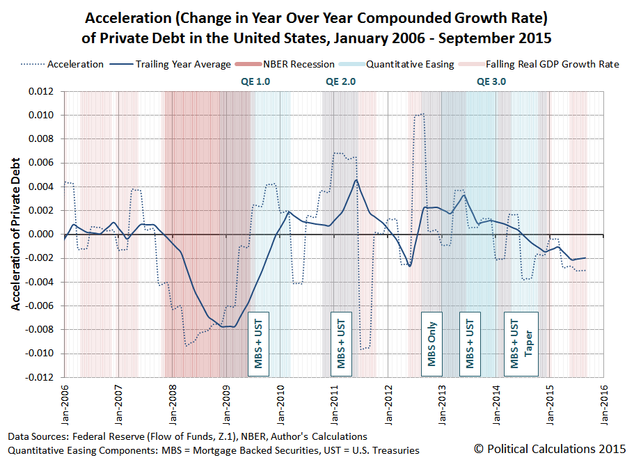
We see that in the third quarter of 2015, the acceleration of private debt in the U.S. remained negative, declining slightly from the previous quarter. Correspondingly, the BEA's second estimate of real GDP for the quarter indicates that its growth rate is likewise falling.

One thing to keep in mind when considering this information is that the U.S. Bureau of Economic Analysis can make significant revisions to its estimates of the nation's GDP during the first several years after it releases its initial estimates as it acquires more accurate and detailed information about the level of economic activity.

For example, the BEA's first estimate for GDP in the third quarter of 2012, released on 26 October 2012 just ahead of the last U.S. presidential elections, indicated that the real GDP growth rate for the quarter was +2.0%, up from the preceding quarter's real growth rate of +1.3%.

But now, according to Table 1 of the BEA's second estimate of GDP for the third quarter of 2015, which was released on 24 November 2015, we find that the real GDP growth rate of 2012-Q3 is now estimate to be just +0.5%, having fallen from the preceding quarter's real growth rate of +1.9%, as the economy of the U.S. was actually in the process of stalling out at that time. Only the U.S. Federal Reserve's expected intervention through its third Quantitative Easing program (QE 3.0), and its boosting effect on private debt, prevented the U.S. economy from fully sinking into recession at that time.

It will be interesting to see how the acceleration of private debt in the U.S. evolves should the Federal Reserve finally follow through on its plans to start hiking short term interest rates in the U.S. in the absence of any additional quantitative easing programs later this week.

Data Sources

U.S. Federal Reserve. Data Download Program. Z.1 Statistical Release (Total Liabilities for All Sectors, Rest of the World, State and Local Governments Excluding Employee Retirement Funds, Federal Government). 1951Q4 - 2015Q3. [Excel Spreadsheet]. Online Database. 10 December 2015. Accessed 14 December 2015.

U.S. Bureau of Economic Analysis. Table 1.1.1. Percent Change from Preceding Period in Real Gross Domestic Product.
1947Q1 through 2015Q3 (second estimate). Online Database]. Accessed 14 December 2015.

References

National Bureau of Economic Research. U.S. Business Cycle Expansions and Contractions. [PDF Document]. Accessed 14 December 2015.

da Costa, Polyana and Ponder, Crissinda. How Fed Moves Affect Mortgage Rates. (Timeline for Federal Reserve Quantitative Easing Programs QE 1.0 through 3.0). [Online Article]. 17 September 2015. Accessed 14 December 2015.

Previously on Political Calculations

Political Calculations. The Position, Velocity and Accelration of Private Debt in the U.S.. 5 November 2015.

Political Calculations. The Correlation Between Decelerating Debt and Falling GDP. 12 November 2015.

Political Calculations. QE and the Acceleration of Private Debt in the U.S.. 18 November 2015.

Earlier this year, economic historian Robert Higgs of the Independent Institute presented a paper challenging the worth of Gross Domestic Product (GDP) as a measure of the economic welfare of a nation's people. In the following excerpt, he gets straight to the heart of the matter in discussing the issues considered by the originators of GDP, such as Simon Kuznets, as they developed it into the statistic we know today.

Among the many issues involved in these developments, none loomed larger than that of the meaning and purpose of national income and product. Analysts eventually settled, for example, on the definition of GDP as the total value at market prices of all final goods and services produced within a nation’s boundaries, usually in a year, although quarterly estimates eventually became routine as well. Once such a number has been produced, however, what does it mean? In particular, is it in some sense a measure of economic welfare? Kuznets, despite many practical compromises in details, had generally sought a measure that in some definite sense could be called a measure of welfare. The parallel developments associated with Richard Stone and others in the United Kingdom, in contrast, forthrightly rejected this interpretation, yet, having done so, they still had to face the question about any given estimate of GDP: What does it mean? Is it simply a hodgepodge of numbers reduced to a single number that in some rough, vague way can be employed to compare one year’s economic performance with another year’s or to compare one country’s performance with another’s? When Kuznets’s approach lost out to the Commerce Department’s, this question was not so much settled as brushed under the rug. Rather than attempt to wrestle with the issue until reaching a definite resolution, economists seemingly tired of debating it and decided simply to forge ahead without worrying much about the meaning of the estimates with which they were working. After all, as they viewed the matter, pressing questions of macroeconomic policy demanded answers, and any particular way of computing GDP would yield a result that can be treated as if it were the economy’s aggregate output—whatever that might mean—for purposes of economic policy making and planning.

Higgs concludes his paper by recognizing that while GDP, as it became, doesn't work very well at all as a measure of the economic welfare of a nation's people. He argues that:

If GDP is to make any sense at all, it must do so in relation to some concept of economic welfare. Economics is not a science of the production of hammers and nails but of wealth—the goods and services that people actually value, as they demonstrate by voluntarily forgoing alternative goods and services in the process of acquiring those they choose to acquire. It is unfortunate that once we recognize this reality, we are left to conclude only that, notwithstanding the disclaimers of nearly all current economists and other analysts who use the NIPA concepts and estimates, GDP is indeed a measure of economic welfare. It is simply an exceedingly poor such measure.

So what would be a better measure? What statistic would provide a much better indication of the economic welfare of a nation's people?

What Would Work Better

Back in March 2015, we more or less stumbled into an answer for the question as we were researching the earliest history of the development of GDP a generation before Kuznets and others began constructing the measure that we know today. We wrote at the time:

In researching the topic, we dug deep into the history of how Gross Domestic Product became the defining measure of a nation's economic performance. Here, the godfathers of GDP were Alfred Marshall and A.C. Pigou, who originally developed the concept of a "National Dividend" or interchangeably, a "National Income" early in the 20th century. Their work was built upon by Simon Kuznets, who actually developed the prototype accounting calculations for GDP as we know it today.

But almost lost in that early history was a very different concept developed by Irving Fisher, who instead of focusing on production as Marshall, Pigou and Kuznets did, defined his concept of the National Dividend around what people consumed. And while Fisher's concept put the focus on the end consumers in a nations, people living in households, where their consumption of goods and services would provide a measure of their quality of life, it was never fully developed because of the challenges that lay in quantifying it....

We see that historically, the main obstacle to making practical use of Fisher's consumption-based definition of the national dividend results from the lack of adequate data to describe the consumption of millions of consumers in the country. But that hasn't been true since 1984, when the U.S. Bureau of Labor Statistics and the U.S. Census Bureau teamed up to conduct the Consumer Expenditure Survey. We actually now have three decades worth of solid data to estimate the money value of total consumption in the hands of millions of consumers in the country. That's something that wasn't possible in the early 20th century when these concepts of National Dividends or National Income were being fleshed out.

We then did what nobody before us had done. We brought Irving Fisher's proposed concept of the national dividend, which would inherently represent a measure of the economic welfare of the nation's people, into reality.

Here are our updated results for the United States as a whole, spanning the years from 1984 through 2014 - the most recent full year for which we have data, in which we've also broken out the aggregate amount of consumption that was funded by debt. Our first chart presents the national dividend in terms of nominal current year U.S. dollars.

Our next chart presents the same data, adjusted for inflation, as given by the Consumer Price Index for All Urban Consumers, to be in terms of constant 2014 U.S. dollars.

Our third chart reveals how our calculation of the national dividend compares to GDP, which reveals both how well GDP reflects the economic welfare of Americans and the extent to which GDP has become a less effective measure of their economic welfare over time.

The preceding charts apply to the United States as an aggregate whole, but if our national dividend calculation is to have value as a measure of the economic well-being of regular Americans, we need to

The National Dividend for the "Typical" American Household

We have the annual average expenditure data to represent what the aggregate national dividend means to the typical U.S. household, or rather, as the data jocks of the U.S. Census Bureau and the U.S. Bureau of Labor Statistics affectionately refer to them in the Consumer Expenditure Survey which collects and presents the data we used to calculate the National Dividend, "consumer units". Our next chart shows the nominal U.S. national dividend per consumer unit for the years 1984 through 2014:

Here is the same information, but now adjusted for the effect of inflation to be in terms of constant 2014 U.S. dollars, in which we discover that there has been little to no material improvement in the economic welfare of the typical U.S. household from 1984 through 2014.

Beyond that observation, we also find that stagnant outcome has been increasingly sustained with an increasing level of household debt over time.

Meanwhile, once we factor in the margin of debt and consider the growing aggregate national dividend in real terms over time with the otherwise flat trajectory of the national dividend per consumer unit/household, we find that the main reason that the aggregate national dividend has increased to the extent that it has is solely because the number of consumer units/households in the U.S. has increased in the years from 1984 through 2014.

Replacing GDP with the National Dividend

Our calculation of the household consumption-based national dividend for the United States reveals a story that runs contrary to the narrative that the producers of GDP have been telling for the last thirty years, while at the same time confirming that GDP is a poor measure of the economic welfare of the American people.

As such, we would suggest that for those looking for an economic statistic that can provide much greater insight into the real economic welfare of the American people, our development of the consumption-based National Dividend is perhaps the most logical place to begin, now that we've made it possible to consider.

Celebrating Political Calculations' Anniversary

Our anniversary posts typically represent the biggest ideas and celebration of the original work we develop here each year. Here are our landmark posts from previous years:

• A Year's Worth of Tools (2005) - we celebrated our first anniversary by listing all the tools we created in our first year. There were just 48 back then. Today, there are nearly 300....
• The S&P 500 At Your Fingertips (2006) - the most popular tool we've ever created, allowing users to calculate the rate of return for investments in the S&P 500, both with and without the effects of inflation, and with and without the reinvestment of dividends, between any two months since January 1871.
• The Sun, In the Center (2007) - we identify the primary driver of stock prices and describe a whole new way to visualize where they're going (especially in periods of order!)
• Acceleration, Amplification and Shifting Time (2008) - we apply elements of chaos theory to describe and predict how stock prices will change, even in periods of disorder.
• The Trigger Point for Taxes (2009) - we work out both when, and by how much, U.S. politicians are likely to change the top U.S. income tax rate. Sadly, events in recent years have proven us right.
• The Zero Deficit Line (2010) - a whole new way to find out how much federal government spending Americans can really afford and how much Americans cannot really afford!
• Can Increasing the Minimum Wage Boost GDP? (2011) - using data for teens and young adults spanning 1994 and 2010, not only do we demonstrate that increasing the minimum wage fails to increase GDP, we demonstrate that it reduces employment and increases income inequality as well!
• The Discovery of the Unseen (2012) - we go where so-called experts on income inequality fear to tread and reveal that U.S. household income inequality has increased over time mostly because more Americans live alone!

We marked our 2013 anniversary in three parts, since we were telling a story too big to be told in a single blog post! Here they are:

• The Major Trends in U.S. Income Inequality Since 1947 (2013, Part 1) - we revisit the U.S. Census Bureau's income inequality data for American individuals, families and households to see what it really tells us.
• The Widows Peak (2013, Part 2) - we identify when the dramatic increase in the number of Americans living alone really occurred and identify which Americans found themselves in that situation.
• The Men Who Weren't There (2013, Part 3) - our final anniversary post installment explores the lasting impact of the men who died in the service of their country in World War 2 and the hole in society that they left behind, which was felt decades later as the dramatic increase in income inequality for U.S. families and households.

Resuming our list of anniversary posts....

• The Toolmaker's Tool (2014) - we make the code we use for creating online tools available to all!
• Replacing GDP with the National Dividend (2015) - we explore our development of an alternative measure of economic welfare that can replace GDP.

References

Chand, Smriti. National Income: Definition, Concepts and Methods of Measuring National Income. [Online Article]. Accessed 14 March 2015.

Higgs, Robert. Gross Domestic Product - an Index of Economic Welfare or a Meaningless Metric. The Independent Review. Volume 20, Number 1, Summer 2015. [PDF Document].

Kennedy, M. Maria John. Macroeconomic Theory. [Online Text]. 2011. Accessed 15 March 2015.

U.S. Bureau of Labor Statistics. Consumer Expenditure Survey. Total Average Annual Expenditures. 1984-2014. [Online Database]. Accessed 19 September 2015.

U.S. Bureau of Labor Statistics. Consumer Price Index - All Urban Consumers (CPI-U), All Items, All Cities, Non-Seasonally Adjusted. CPI Detailed Report Tables. Table 24. [Online Database]. Accessed 19 September 2015.

U.S. Bureau of Economic Analysis. National Income and Product Accounts Tables. Table 1.1.5. Gross Domestic Product. [Online Database]. Accessed 19 September 2015.