Scandal erupted on the Australian edition of The Bachelor when the Bachelor, 32-year old astrophysicist Matt Agnew, asked 28-year old chemical engineer Chelsea McLeod to solve math problems in order to find the combination numbers of a safe on their third and final date before the show's conclusion.
We're not making this up. Here's a video excerpt from the show:
The task greatly upset the show's fan base. Here's the story from the Daily Mail:
Since day one, Bachelor Matt Agnew has embraced the fact Chelsie McLeod shares his same passion for science.
But fans were left confused during the pair's final date on Wednesday's semi-final, as the astrophysicist, 32, tasked the chemical engineer, 28, with math equations.
'This would literally be my worst nightmare!' one fan Tweeted, after Matt described the maths problem as a 'fun activity' for Chelsie to complete.
'I cannot believe you're making me do this right now!' Chelsie said to Matt, which viewers appeared to agree with.
Matt handed Chelsie a pen and paper to solve a math problem to open a safe, which housed a present for the star.
At least it ended well. Chelsie correctly solved the math problems, determined the combination to the safe, and revealed the prize:
After cracking equations, Chelsie typed in the code which opened to a box with a necklace engraved with the chemical formula for oxytocin.
The formula was a reference to their first meeting on the red carpet where she gave him a temporary tattooed of the same chemical.
'So you got to put some oxytocin on my chest, to my heart, and this way, the necklace, it'll be close, some oxytocin near your heart as well.
It's probably no surprise that the two ended up together in the aftermath of the show's suitably romantic final rose ceremony.
But more than just a triumph of math and love, the episode demonstrates assortative mating in action, where couples come together because of their shared potential in addition to their shared attraction. Which in the case of their shared potential, more often than not also reflects their shared earning potential.
But since most couples don't have the accelerated contrivances of a televised dating show to utilize during their courtships, how does that tend to work in the real world?
Alparslan Tuncay described how couples made up of individuals with similar earnings potential come often come together in a paper Marginal Revolution's Tyler Cowen described as "the best results on assortative mating and inequality I have seen". Here's the abstract:
This paper studies the evolution of assortative mating in the permanent wage (the individual-specific component of wage) in the U.S., its role in the increase in family wage inequality, and the factors behind this evolution. I first document a substantial trend in assortative mating, as measured by the permanent wage correlation of couples, from 0.3 for families formed in the late 1960s to 0.52 for families formed in the late 1980s. I show that this trend accounts for more than one-third of the increase in family wage inequality across these cohorts of families. I then argue that the increase in marriage age across these cohorts contributed to the assortative mating and thus to the rising inequality. Individuals face a large degree of uncertainty about their permanent wages early in their careers. If they marry early, as most individuals in the late 1960s did, this uncertainty leads to weak marital sorting along permanent wage. But when marriage is delayed, as in the late 1980s, the sorting becomes stronger due to the quick resolution of this uncertainty with work experience. After providing reduced-form evidence on the impact of marriage age, I build and estimate a marriage model with wage uncertainty and show that the increase in marriage age can explain almost 80% of the increase in assortative mating.
Marrying later contributes to this outcome because it allows the each partner in a couple the time to demonstrate their earning capacities, which would either reinforce the pairing or lead to a break up if the two are incompatibly mismatched. Tuncay's findings confirm what we've seen in the data for income inequality in the United States over that period of time, where there has been no change in the income inequality level for individuals, but a rising trend for both households and families as a greater emphasis on college education and early career establishment before marriage has become common in American society since the 1960s.
Assortative mating provides a very reasonable explanation for these outcomes. And we've just seen it at work, in all its oxytocin-enhanced sweetness, on The Bachelor Australia.
Labels: demographics, income inequality, math


We've drilled down a bit deeper into the U.S. Census Bureau's data documenting the lifetime income trajectories that Americans have expect based on their level of education.
Previously, we looked just at those trajectories for all Americans with some work experience for the years from 2000 through 2016, which includes the data for Americans who work part time, who may only work part of a year, who may have exited the workforce, whether temporarily, such as to focus on raising children or because of layoffs or other job changes, or permanently, such as through retirement.
Now, we're focusing like a laser beam on Americans who work full-time, year-round and, as a bonus, we've expanded the data in our analysis to include all the years for which the Census Bureau has provided this information in a convenient digital format, which is to say since 1994. Our first chart shows the mean lifetime income trajectories for various levels of educational attainment for these full-time, year-round workers:

This chart reveals a clear difference in the education level-based lifetime income trajectories that Americans who work full-time, all year-round, where those who can sustain working at this pace can expect to have, on average, higher lifetime incomes with higher levels of educational attainment.
That income differentiation also carries from the very outset of their adult working lives, where incomes rise with higher levels of education. The following chart shows this data for 2016, which until September 2018 when the data for 2017 will be made public, represents the most recent year for which this data is available.

The pattern shown in the first chart is persistent from year-to-year in the Census Bureau's historical data, which provides confidence that the survey data is capturing the average lifetime income trajectories of Americans who work full-time, year-round. As an example of this persistence, the following chart shows the age-based incomes as a percentage of the mean income of the Age 18-24 cohort for Bachelor degree holders who work full-time, year-round.

While there is considerable variation from year to year, the overall pattern for lifetime income trajectories holds across the various levels of educational attainment and over what is now more than two decades worth of income data.
References
U.S. Census Bureau. Current Population Survey Tables for Personal Income. PINC-04. Educational Attainment--People 18 Years Old and Over, by Total Money Earnings, Work Experience, Age, Race, Hispanic Origin, and Sex. Both Sexes, All Races. Worked Full Time, Year Round. [Digital files: 1994, 1995, 1996, 1997, 1998, 1999, 2000, 2001, 2002, 2003, 2004, 2005, 2006, 2007, 2008, 2009, 2010, 2011, 2012, 2013, 2014, 2015, 2016]. Accessed 19 August 2018.
Labels: data visualization, demographics, education, income, income inequality
What are the differences between the Congressional Budget Office's estimates of income inequality among U.S. households and the annual estimates produced by the U.S. Census Bureau?
We've taken a stab at answering that question in a visual format through the following infographic! Please click the image to access a larger, more readable version of the chart to get the quick run-down on what makes each of the indicated estimates different from one another, while also checking out over 50 years worth of U.S. household income inequality data as measured by the estimable Gini ratio.

As for Item 4, we'll have more information soon, but as a quick indication of what we can do with the Census data that cannot be done with the CBO's data, check out our tool What Is Your Income Percentile Ranking?
Data Sources
Congressional Budget Office. The Distribution of Household Income and Federal Taxes, 2013. [PDF Document]. Supplemental Data [Excel Spreadsheet]. June 2016.
U.S. Census Bureau. Current Population Survey. Annual Social and Economic Supplements. Historical Income Tables: Households Table H-4. Gini Ratios for Households, by Race and Hispanic Origin of Householder. All Races. [Excel Spreadsheet]. 10 August 2017.
Labels: data visualization, income distribution, income inequality
According to data published in December 2014 by the U.S. Bureau of Labor Statistics in its annual Highlights of Women's Earnings report, in 2013, women made up 48.2% of the total number of workers in the U.S. labor force and the average woman in the United States earned 76% of what the average man did.
Also according to the same BLS report, going by the usual number of hours worked each week, the median earnings for women in the U.S. was within 10% of those for men for all but two categories: people who work 60 or more hours per week and also people who work 35 or more hours per week, but whose hours vary considerably from week to week.
Meanwhile, it would appear that U.S. men are paid more to work longer hours, but that U.S. women are paid more to work fewer hours.
But you don't have to take our word for it! Here's the data straight from Table 5 of the report for the number of workers by sex for each category of the usual number of hours worked each week:
| 2013: Number of Workers by Sex and Usual Number of Hours Worked Each Week | |||
|---|---|---|---|
| Hours Worked per Week | Number of Workers | Number of Women | Number of Men |
| 1 to 4 hours | 520,000 | 338,000 | 182,000 |
| 5 to 9 hours | 1,155,000 | 771,000 | 383,000 |
| 10 to 14 hours | 1,785,000 | 1,168,000 | 617,000 |
| 15 to 19 hours | 2,604,000 | 1,760,000 | 844,000 |
| 20 to 24 hours | 6,654,000 | 4,307,000 | 2,347,000 |
| 25 to 29 hours | 3,200,000 | 2,081,000 | 1,120,000 |
| 30 to 34 hours | 6,268,000 | 4,035,000 | 2,232,000 |
| Hours Vary (usually < 35 hours) | 2,478,000 | 1,500,000 | 978,000 |
| 35 to 39 hours | 8,128,000 | 5,380,000 | 2,748,000 |
| Hours Vary (usually 35 or more hours) | 5,427,000 | 2,060,000 | 3,367,000 |
| 40 hours | 70,466,000 | 32,504,000 | 37,963,000 |
| 41 to 44 hours | 1,031,000 | 390,000 | 642,000 |
| 45 to 48 hours | 5,493,000 | 1,957,000 | 3,536,000 |
| 49 to 59 hours | 9,119,000 | 2,805,000 | 6,314,000 |
| 60 or more hours | 4,599,000 | 1,173,000 | 3,426,000 |
| All | 129,110,000 | 62,316,000 | 66,794,000 |
And here's the corresponding data from the same table as it relates the median weekly earnings by the usual number of hours worked each week:
| 2013: Median Weekly Earnings by Sex and Usual Number of Hours Worked Each Week | |||
|---|---|---|---|
| Hours Worked per Week | Median Weekly Earnings (Both Sexes) | Median Weekly Earnings (Women) | Median Weekly Earnings (Men) |
| 1 to 4 hours | $58 | $56 | $61 |
| 5 to 9 hours | $75 | $76 | $74 |
| 10 to 14 hours | $113 | $115 | $109 |
| 15 to 19 hours | $159 | $163 | $151 |
| 20 to 24 hours | $205 | $202 | $210 |
| 25 to 29 hours | $217 | $223 | $209 |
| 30 to 34 hours | $264 | $270 | $255 |
| Hours Vary (usually < 35 hours) | $336 | $352 | $315 |
| 35 to 39 hours | $495 | $507 | $466 |
| Hours Vary (usually 35 or more hours) | $672 | $496 | $791 |
| 40 hours | $732 | $691 | $771 |
| 41 to 44 hours | $880 | $841 | $912 |
| 45 to 48 hours | $1,054 | $993 | $1,097 |
| 49 to 59 hours | $1,270 | $1,193 | $1,317 |
| 60 or more hours | $1,373 | $1,202 | $1,436 |
| All | $665 | $584 | $764 |
We thought it might be interesting to visualize all the data we've presented in table form above in a single chart. To do that, so we can show all the data with a single axis, we've calculated the percentage of all workers that are women along with the percentage of men's median weekly earnings that women earn for each category of usual hours worked per week.

What we see is that the median U.S. woman is typically being paid a 10% premium to work part time compared to a U.S. man working the same number of hours each week. As you can imagine, that kind of financial incentive would go a very long way to explaining why two-thirds of all working Americans who work less than 40 hours per week are women.
But as the number of usual hours worked each week rises, we see that situation reverses. For people who regularly work 40 up to 59 hours per week, women earn about 90% of what a man working the same number of hours does. However, as the number of hours required to earn incomes rise, we also see that fewer and fewer women are to be found working. At the topmost end, we see that for people who work 60 or more hours per week, the median income earned by a woman drops to 84% of the median working earnings of a man who puts in those kinds of hours, and also that only 26% of the total number of people who spend more than half their waking hours per week working at income-paying jobs like this are women.
U.S. women would also appear to be highly averse to working variable numbers of hours each week, which we see in the dips for the percentage share of workers who work varying hours each week with respect to those who work a steady number of hours.
While it is the combination of all these factors that results in the median weekly earnings for American women being just 76% of those for men, we find that it is the relatively higher pay rewards of part time employment for women as compared to men and the relative absence of women who choose to work 60 or more hours at income-paying jobs each week that are the greatest contributors to that statistic.
Data Source
U.S. Bureau of Labor Statistics. BLS Report 1051: Highlights of Women's Earnings in 2013. Table 5. Median usual weekly earnings of wage and salary workers, by hours usually worked and sex, 2013 annual averages. [PDF Document]. December 2014.
Labels: demographics, income, income inequality

What if income inequality theorists got their way and stopped income inequality from ever increasing? What would be the result of that kind of achievement?
We came across the results of a unique experiment that was conducted nearly 100 years ago that answers the question, where a predefined level of income inequality was strictly enforced upon a small group of individual laborers with an outcome that permanently affected not just their jobs but also a national institution.
The experiment was unknowingly conducted by the professional baseball team owner Charles Comiskey, who after assembling "the best team money could buy", ultimately produced the most significant act of corruption in American sports history as a direct result of his strict enforcement of a policy of income equality upon his players regardless of their talent or individual contributions to the team's success: the Chicago Black Sox Scandal, in which a number of players on the 1919 Chicago White Sox deliberately lost the 1919 World Series to the Cincinnati Reds in return for payoffs from professional gamblers looking to gain from advance knowledge of the outcome.
Bruce Lowitt describes how the equality of income imposed by Charles Comiskey actually generated the worst possible outcome for everyone involved:
There was good reason the Sox were susceptible to the lure of quick money. They were among the American League's best players but Charles Comiskey paid most of them no more than the worst. The promised bonus for winning the 1917 pennant was a case of cheap champagne. Before the 1919 season, Comiskey promised Cicotte an extra $10,000 if he won 30 games. When Cicotte reached 29, Comiskey benched him. Player resentment was rampant.
Here, we see a prime example of the extreme penalty that Comiskey imposed upon one of his star players, pitcher Eddie Cicotte, to ensure that he would not ever be paid any more than any other player on the team, as Comiskey effectively imposed a 100% marginal income tax upon Cicotte as he came too close to becoming too successful in Comiskey's eyes.
What happened in response to that event would ultimately and permanently change America's national pastime as that achievement in preventing an increase in income inequality inspired acts of extreme corruption by eight players on the team, who wanted to have their pay reflect their real relative level of productivity and contribution to the team's success. And by "extreme corruption", we're not kidding. They threw the World Series, deliberately losing to the Cincinnati Reds in return for payoffs from professional gamblers.

But what's really curious is what happened after the World Series ended, because it was some time before the scandal was sorted out. Here, seven of the players involved in the scandal were signed to new contracts with the White Sox to play for the team in 1920, the year after the scandal, where they received anywhere from a 21% to a 100% increase in their previous year's salaries.
That's an especially curious thing because it is clear that Charles Comiskey was aware that the seven players had very likely deliberately lost the 1919 World Series before the contracts were negotiated. He could have refused to negotiate with the players suspected of corruption, but instead, he recognized that his previous policy for more equalized player pay was an abject failure and gave in to the greater level of income inequality demanded by the players in return for their real contributions to the team's success.
In 1919, the salaries for these seven players had ranged between a low of $2,750 to $6,000, a spread of $3,250, with the top income set at 218% of the income of the lowest paid player involved in the scandal. But in 1920, the player's incomes ranged from $3,200 to $10,000 (for Cicotte, who was paid $5,000 in 1919): a spread of $6,800, more than double what it had been in 1919, with the top income growing to be 312% of the lowest.
The Chicago White Sox went on to finish second in the American League in 1920, as the team's hitting and pitching was strong, finishing just two games behind the Cleveland Indians who had a stellar year. Increasing the income inequality among the team's players did not harm their performance as they achieved honest success - even winning eight more games than they had in the 1919 season (the 1920 season was 14 games longer than the 1919 season).
That's the benefit of increasing income inequality - a more honest system for rewarding the real contributions of the most productive members of a society. The penalties imposed by a system that rigorously imposes equality will almost invariably lead to corruption.
After the 1920 season, the news of the scandal broke break wide open, with the ultimate outcome that the eight Chicago White Sox players who had participated in the conspiracy to deliberately lose the 1919 World Series were banned from the sport of baseball for life, as the league's new, indepedent commissioner took actions to eliminate the potential influence that gambling could have in order to boost the sport's integrity.
But that is a whole separate issue from what really caused the scandal!
Labels: income inequality, sports

Now that we've established what the relative purchasing power of a dollar is in each of the United States, we're going to apply that information today to solve one of the great problems of our time: how to set the minimum wage in each state in order to achieve purchasing power equality.
After all, it goes against the ultimate liberal ideals of fairness and equality of outcomes if, thanks to nothing other than the relative cost of living in each state, that a minimum wage earner in Mississippi is able to buy more things with their earnings than can a person earning the identical wage in a high cost of living state like New York.
Clearly, in the interest of fairness and of achieving purchasing power equality, the minimum wage in each state needs to be adjusted in such a way that a person who earns the minimum wage in each state can buy no more and no less than the same amount of real goods and services. That's the great problem for society that we'll be solving today.
Let's start by examining the applicable minimum wage that applies to each state in 2012, the year for which we have the relative purchasing power data, which is the greater of either the state's own minimum wage or the federal minimum wage of $7.25 per hour. That data is directly encoded in the interactive map below:
Next, let's calculate what each state's minimum wage would have to be so that the individual's who earn it will have an equal amount of purchasing power, regardless of the state in which they might live. Here, we've used the federal minimum wage of $7.25 per hour as the benchmark for calculating the minimum wage levels in each state that would achieve purchasing power equality across the entire nation.
Finally, we calculated how much each state would need to adjust their minimum wage levels in order to realize the very achievable dream of purchasing power equality for minimum wage earners throughout the United States.
What this exercise demonstrates is that if one really cares about achieving equality, it makes absolutely no sense to impose a national minimum wage, which we observe produces the situation where the minimum wage earners in some states are considerably worse off than individuals earning the same wage in lower cost of living states - the very essence of income inequality and unfairness.
Labels: data visualization, economics, income inequality, minimum wage, satire
According to the Associated Press, the typical Chief Executive Officer of a company makes 257 times the average worker's salary.
Is that really a problem?
Here's why we ask that question - how much somebody earns in doing a job depends tremendously on who else can do their job. For example, people who earn the minimum wage tend to have minimal job responsibilities. Consider the case of Tyree Johnson, a 20-year McDonalds employee:
After 20 years cooking burgers and manning the fryer for the national chain, Tyree Johnson still makes just the minimum wage, Bloomberg reports. That's $8.25 an hour in 44-year-old Johnson's hometown of Chicago, where he works at two different McDonald's restaurants.
First, let's look at what it would take to replace Tyree Johnson as a fry cook at McDonalds. Here's a recollection of a St. Louis McDonalds' crew member's experience in being hired and trained:
I applied in-person and the process took a day - interviewed at McDonald's in March 2013.
Interview Details – The interview process took less than 15 minutes. It wasn't really thorough or relevant. Once hired, you go through a two day training period. It was a group interview and not hard at all.
Negotiation Details – You got to choose the hours you worked and they attempted to make a flexible schedule.

Of course, one of the big reasons that so little training is needed is because McDonalds invests heavily in automating many aspects of restaurant work, with the position of cashier likely to be the next job at McDonalds that will make more sense to have done by technology rather than by people. As a business, McDonalds does not rely upon employing workers at minimal wages for its profits, as it long ago recognized that standardizing and automating work was its key to growth. Consequently, McDonalds employees earn wages consistent with those who might replace them in their very limited roles.
By contrast, a CEO is responsible for overseeing the operations at all levels of a company's operations and all locations at which the company does business. The CEO is responsible for all aspects of the company's business strategy and is responsible for reporting on the state of the business to the company's owners, which in many cases, includes themselves. Generally speaking, a CEO is not easily replaceable, taking months to put into place, at a minimum.
In 2012, McDonald's CEO Jim Skinner earned $8.75 million. He retired and was replaced by Don Thompson in June 2012, who had joined McDonalds 22 years earlier, leading projects to design and develop robotic equipment for food transport and control circuits for automating cooking operations at McDonalds' 34,000+ restaurants worldwide. Thompson had been being groomed to become McDonald's CEO since being promoted to be the company's Chief Operating Officer in June 2010. In 2013, Thompson earned $9.5 million as CEO.
We're making a point of emphasizing the sheer scope of McDonalds' operations because that's the key to understanding what drives the pay of CEOs.
Xavier Gabaix and Augustin Landier found back in 2008 (using data up through 2003) that CEO pay follows a special version of a power law, known as Zipf's Law, where what a major company's CEO earns is directly proportional to the size of the firm that they are responsible for running. The chart below shows the correlation between firm size and CEO compensation for the top 500 public firms in 2010:

But more importantly, Gabaix and Landier have updated their earlier results to include data through 2011, allowing them to determine whether the relationship between firm size and CEO compensation would hold through the extreme gyrations the economy experienced in going from boom, to bust and then into recovery. Here's the abstract of their 2013 paper updating their findings:
In the 'size of stakes' view quantitatively formalised in Gabaix and Landier (2008), CEO compensation reflects the size of firms affected by talent in a competitive market. The years 2004-2011 were not part of the initial study and offer a laboratory to examine the theory with new positive and negative shocks. Executive compensation (measured ex ante) did closely track the evolution of average firm value, supporting the 'size of stakes' view out of sample. During 2007 - 2009, firm value decreased by 17%, and CEO pay by 28%. During 2009-2011, firm value increased by 19% and CEO pay by 22%.
We see then that CEO pay is indeed driven by firm size.

In fact, the only time we see CEO compensation race far above what we would expect based upon firm size directly corresponds to the years of the Dot-Com Bubble, where a reduction in the capital gains tax rate without a corresponding reduction in dividend tax rates created massive distortionary imbalances in the U.S. economy. Imbalances, we might add, affected people earning minimum wages by just as much as those who pocketed that era's massive capital gains.
And for those people whose pay is determined by the wages that would be paid to their potential replacement, perhaps a good question to ask is what can you do to generate enough additional revenue to justify a higher paycheck for yourself without passing the costs on to your customers. Because the odds are that the CEO of the company where you work already has some idea of what that answer might be.
And you know that they've just gotta be loving it!
References
Xavier Gabaix & Augustin Landier & Julien Sauvagnat, 2014. "CEO Pay and Firm Size: An Update After the Crisis," Economic Journal, Royal Economic Society, vol. 124(574), pages F40-F59, 02. http://www.nber.org/papers/w19078. [Ungated Version].
Political Calculations. Debunking Income Inequality Theory. http://politicalcalculations.blogspot.com/2014/01/debunking-income-inequality-theory.html. 23 January 2014.
Political Calculations. What Caused the Dot Com Bubble to Begin and What Caused It to End? http://politicalcalculations.blogspot.com/2010/12/what-caused-dot-com-bubble-to-begin-and.html. 15 December 2010.
Labels: business, income inequality, jobs
January 2014 is not shaping up to be a good month for the reality-challenged belief system of the Incredibly Incurious Journalist Jonathan Chait.
Still smarting from his defeat in the debate on whether Obamacare is beyond rescue, the findings of newly published academic research into the nature of why income inequality among U.S. households and families has risen over time couldn't have come at a worst time for the leftist journalist.
The abstract of the paper gets straight to the issue at hand:
Has there been an increase in positive assortative mating? Does assortative mating contribute to household income inequality? Data from the United States Census Bureau suggests there has been a rise in assortative mating. Additionally, assortative mating affects household income inequality. In particular, if matching in 2005 between husbands and wives had been random, instead of the pattern observed in the data, then the Gini coefficient would have fallen from the observed 0.43 to 0.34, so that income inequality would be smaller. Thus, assortative mating is important for income inequality. The high level of married female labor-force participation in 2005 is important for this result.
"Assortative mating" is a term borrowed from genetics, which refers to when the members of a species select mates based on their observable characteristics, seeking mates whose characteristics are either similar to their own or that they find desirable.
Where economics and income inequality come into play is when one of the main characteristics that people use to form families and households is the income-earning potential of their prospective spouse. Our own groundbreaking analysis shows how simply combining working or non-working men and working or non-working women into various one or two-person households can create considerable disparity in the amount of income earned by each resulting household:
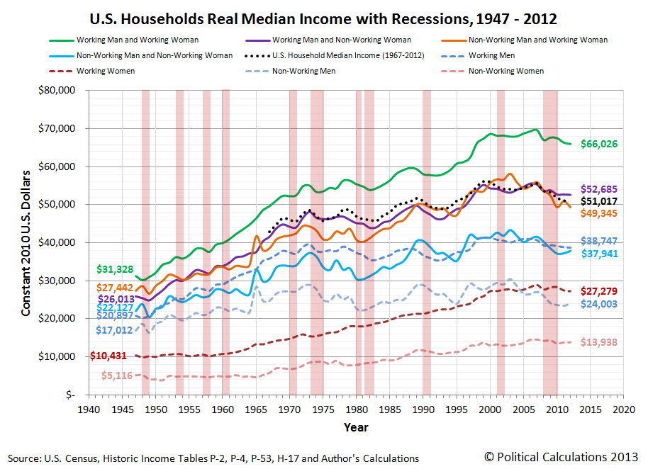
The data in this chart is solely based on the median income earned by each type of household member, so every individual income upon which it is based is represented by a person whose income places them in the exact middle of the income distribution for their category in the year indicated.
Now, consider the following changes in the composition of households might change as a result of this assortative mating. What would happen to the measured amount of income inequality over time if:
- Men and women who both have high income earning potential increasingly form households together, with both delivering on that potential.
- Men and women who both have low income earning potential increasingly form households together, with both delivering on that potential.
Why, that's a recipe for increasing income inequality over time, isn't it? Especially when you consider these changes would coincide with a reduction in the number of households and families that are composed of one individual with high income-earning potential and one individual with low-income earning potential.
And that doesn't even consider the situation for when a household or family either fails or if one of the income-earning members of the household passes away, leaving behind just a single income-earning household.
All of which combines to produce the following picture for the major trends in income inequality since 1947:

In this chart, we see that the measured income inequality among individual Americans hasn't meaningfully changed since 1960, while the income inequality measured in American households and families has increased. That is the telltale indication that social factors, rather than economic ones, are behind the increase in the income inequality observed for U.S. households and families.
This is the kind of real world evidence that income inequality theorists like Chait and his precious few sources in academia who share his cloistered world view disregard. Because if they accepted it, they would have to abandon the policy prescriptions that derive from their debunked claims.
But then, we're talking about someone who actually believes that Obamacare can be rescued. Even though the evidence today says that it cannot, especially considering that the whole political rationale for the program was sold on lies. Lies fully bought into by people like today's income inequality theorists.
And for the record, Jonathan Chait has still never contacted us regarding any of the original analysis we've generated here on the topic of the income distribution of Americans over the years. As journalists go, he's certainly an incredibly, unbelievably, stupendously, incurious member of the profession.
What else can we say? Vindication tastes sweet! Our long-time readers know what comes next....
Previously on Political Calculations
- How to Detect Junk Science
- Debunking Income Inequality Theory
- The Incredibly Incurious Journalism of Jonathan Chait
- The Continuing Adventures of an Incredibly Incurious Journalist
- The Major Trends in U.S. Income Inequality Since 1947
- The Discovery of the Unseen
- The Real Story Behind "Rising" U.S. Income Inequality
- Low End Income Inequality in the U.S.
Labels: income inequality
Income inequality theory is a lot like ancient astronaut theory, in that in order to believe in it, you have to disregard a lot of evidence to the contrary.
Let's start with the most basic premise of income inequality theory: that when the rich become richer, the poor become worse off.
Do they really?
Today, we're going to revisit a time in recent American history that income inequality theorists claim represents a peak in the degree of economic inequality in the nation, where income became highly concentrated in the hands of just a lucky few, leaving millions of the poorest Americans at the lowest end of the income spectrum worse off.
And we're going to do that by comparing the top to the bottom, during the days of the Dot-Com Bubble.

Perhaps no other episode in modern American history so clearly separated the people at the top of the income earning spectrum, who raked in millions upon millions from the capital gains associated with a booming stock market that rose to spectacular new heights, and the people at the bottom, whom we'll represent by the people with the least education, least skills and least work experience in the U.S. economy: Americans between the ages of 16 and 24!
The Highest of the High
Although we normally date the beginning of the Dot-Com Stock Market Bubble to the month of April 1997 [1], in reality, that bubble really began to inflate on Wednesday, 7 May 1997.
The action that caused the prices of stocks to suddenly start rising rapidly was the announcement that day that the Tax Relief Act of 1997 would incorporate a major reduction in the tax rate for capital gains, which would be retroactive to 7 May 1997 after the act was signed into law.
Because the tax rate for dividends wasn't similarly reduced, the disparity that was introduced in potential after-tax returns for investors sparked off the inflation phase of the Dot Com Bubble. Investors quickly bid up stock prices, and especially the stock prices of companies that didn't pay stock-price reducing dividends, as they could realize greater after-tax returns that way.
An adverse feedback cycle soon developed, amplifying the inflation of the bubble, which continued boosting stock prices up to its unsustainable August 2000 peak. After which, the Dot Com Bubble entered its deflation phase, which lasted until the tax rates for dividends and capital gains were set to be equal to each other by the Jobs and Growth Tax Relief Reconciliation Act of 2003, which was signed into law on 28 May 2003, marking the end of the Dot Com Bubble.
The best way to see how out-of-the-ordinary the Dot Com Bubble was is to track its growth with respect to the dividends per share that the stock market generated during that period of time, and to compare it to the trends that came before and after. We've done that for the annual averages for the S&P 500 in the chart below, which we've also adjusted for inflation to be in terms of constant year 2000 U.S. dollars, since that year marks the peak for the Dot Com Bubble.

In the years in between 1997 and 2003, the investors who sold the stocks they owned during that time became the people whose growing income from those tax-cut fueled capital gains quickly put them in the stratosphere of the U.S. income distribution, as more income became concentrated [2] among these topmost income earners than in the several decades preceding the bubble's peak.
These individuals then represent the highest of the high. The very people into whose hands the most income was concentrated during the years of the Dot Com Bubble.
The Lowest of the Low
Meanwhile, the people at the bottom of the U.S. income spectrum would be earning the minimum wage. Since approximately half of the people who populate the lowest end of the income spectrum in the U.S. are between the ages of 16 and 24, we can use this portion of the population to demonstrate how they fared during this period of time.
To do that, we'll return to our recently updated minimum wage demand curve for this portion of the U.S. income earning population, updating it to also be in the inflation-adjusted terms of constant year 2000 U.S. dollars.

Notice that during the years of the Dot-Com Bubble that the number of Age 16-24 Americans with incomes swelled far above where our minimum wage demand curve says should have happened. At its peak in the year 2000, we estimate that over 1.6 million U.S. teens and young adults were earning incomes than would have been possible without the Dot Com Bubble's effect on the U.S. economy.
But that's not the most remarkable observation that we are now able to make.
Debunking Income Inequality Theory
What would happen if we overlayed these two charts? Remember, the first chart showing the trajectory of stock prices during the Dot Com Bubble directly indicates the outsized income gains that the people at the highest end of the U.S. income spectrum accumulated during the years that saw the greatest increase in income inequality in American history up to that point.
The second chart shows what happened for the people at the very bottom of the U.S. distribution income during those same years. We've already observed that far more people in this group would appear to have earned income during this time than would have been predicted by the data outside the period of the Dot Com Bubble, but how much worse off did they fare?

This is the chart that completely debunks the main premise of income inequality theory - that the rich get richer at the expense of the poor, who income inequality theorists claim get poorer.
What we've revealed is that the gains of the people at the bottom were directly proportional, or nearly so, to the gains of the people at the top during the Dot Com Bubble.
The people at the top saw those gains in the form of income acquired through investments in the U.S. stock market. The people at the bottom saw those gains in the forms of jobs that allowed millions more to earn incomes through wages and salaries, many at jobs that paid at or near the minimum wage, than they could if the economic activity generated during the years of the Dot Com Bubble did not occur.

The effect on the income inequality math is pretty straightforward - the Dot Com Bubble both put a lot of money into the hands of the people at the top of the income spectrum, while at the same time, it supported a very large influx of people at the bottom - people who wouldn't have been included in the calculation of income inequality if they had no income at all.
But they did - with these millions of these additional people in the U.S. workforce earning billions of dollars.
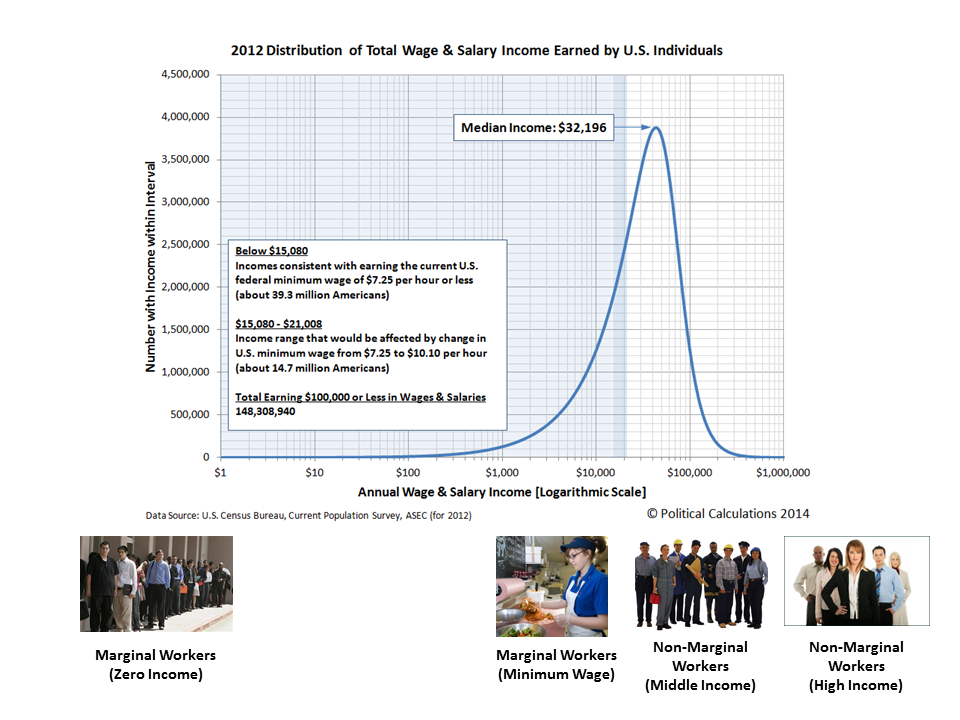
The only way this effect wouldn't play out is if the minimum wage were raised so high, it would effectively block employers from being able to hire marginally educated and experienced Americans because these individuals would not be able to generate enough revenue to cover the costs of employing them. As we can see in the charts above, the Dot Com Bubble generated enough additional economic activity to more than offset the negative effect of the minimum wage increases during that time. Alas, economic bubbles are not sustainable.
The alternative for these most economically marginal of Americans is to not participate in the U.S. job market at all and to earn zero income as a result.
During the Dot Com Bubble that was a choice. Perhaps such people who chose not to earn incomes instead chose to attend school and obtain masters and doctorate degrees in fields that just don't provide much of an economic return on their investment, so they saw no gains from the bubble-driven economy of the late 1990s or early 2000s. We strongly suspect that these particular individuals, along with their academic mentors who likewise were on the economic sidelines, are today's leading income inequality theorists.
It occurs to us that the main difference between income inequality theorists and ancient astronaut theorists is that the ancient astronaut theorists have more credibility.
Footnotes
[1] We follow the same practice for dating the beginning and end of stock market events that the National Bureau of Economic Research follows in determining when recessions begin and end. Here, the NBER doesn't select the month in which the economy actually begins to contract as the starting point for a recession, but rather the month in which the previous period of economic expansion peaked.
Following the same logic with monthly stock price data, we've identified April 1997 as the starting month for the Dot Com Bubble since stock prices began to deviate sharply from their previously established trajectory in May 1997. April 1997 then may be thought of as the starting month, or rather, Month 0 of the Dot-Com Bubble.
[2] The concentration of income at the top end of the U.S. income spectrum during the Dot-Com Bubble is clearly evident in Figure 2 of the material introduced here by Victor Yakovenko. There's a second period of income concentration later with the U.S. housing bubble, but as we've previously shown in a three part series (Part 1, Part 2, Part 3), that was just the result of a capital flow from one market to the other....
Image Credits: Michael Wu.
Previously on Political Calculations
We celebrated our 2013 anniversary in three parts, since we were telling a story too big to be told in a single blog post! Here they are:
- The Major Trends in U.S. Income Inequality Since 1947 (2013, Part 1) - we revisit the U.S. Census Bureau's income inequality data for American individuals, families and households to see what it really tells us.
- The Widows Peak (2013, Part 2) - we identify when the dramatic increase in the number of Americans living alone really occurred and identify which Americans found themselves in that situation.
- The Men Who Weren't There (2013, Part 3) - our final anniversary post installment explores the lasting impact of the men who died in the service of their country in World War 2 and the hole in society that they left behind, which was felt decades later as the dramatic increase in income inequality for U.S. families and households.
Meanwhile, there were the things that led up to those findings:
- Can Increasing the Minimum Wage Boost GDP? (2011) - using data for teens and young adults spanning 1994 and 2010, not only do we demonstrate that increasing the minimum wage fails to increase GDP, we demonstrate that it reduces employment and increases income inequality as well!
- The Discovery of the Unseen (2012) - we go where so-called experts on income inequality fear to tread and reveal that U.S. household income inequality has increased over time mostly because more Americans live alone!
- The Major Trends in U.S. Income Inequality Since 1947 - want to know why you cannot blindly rely on the data that income inequality theorists use to make their case?
- The Real Story of "Rising" U.S. Income Inequality - we find that social factors, rather than economic ones, account for virtually all of the claimed increase in income inequality over time.
- Twenty Years of the U.S. Minimum Wage - we introduce our updated minimum wage demand curve, complete with a tool you can use to anticipate how the income-earning prospects for Americans between the ages of 16 and 24 will change as a result of a change in the U.S. minimum wage.
- The Income Distribution of U.S. Wage and Salary Earners in 2012 - the most recent snapshot we have of how income is distributed in the U.S. among those who earn wages or salaries!
Labels: economics, income distribution, income inequality, minimum wage, SP 500
What is the lasting economic impact of the men who died while serving their country in war?
In our last installment, we showed that the single greatest factor behind the exponential increase in the number of single person households after the 1930s was the loss of over 416,000 men who died while in military service during the Second World War. The vast majority of these men had been drafted into military service, all between the ages of 18 and 37, where they were inducted after being selected through a lottery process operated by their local draft boards.
That lottery process ensured that approximately equal numbers of healthy American men by year of birth would enter into military service, which explains why the average age of the men who served in the U.S. military during World War 2 was 26. And since over 87% of U.S. military casualties in the war occurred in 1944 and 1945, enough time had elapsed from when President Franklin D. Roosevelt imposed the draft by executive order for the population of American casualties to reflect the age distribution of those who had been drafted.

If these more than 416,000 men had lived, they would have turned Age 65 in the years from 1970 through 1992. Instead, if we assume that the number of American casualties are approximately equally distributed by age, reflecting the age distribution of those who served, beginning in 1970 at least 15,735 fewer men reached Age 65 in each year for the next 22 years than would have been the case otherwise. (87% of the over 416,000 deaths of U.S. servicemen during the war is 361,920, which divided by the 23 years between 1970 and 1992, works out to be 15,735 men per year.)
The Hole They Left Behind in American Society
How can you measure the economic impact of men who died?
The only way that can really be done is to measure the size of the hole they left behind in society. Here, that hole can be measured by the population of women who lost their husbands and boyfriends, who because the number of women outnumbered the number of men after the end of the war, meant that many would have to go on to either live with their families or alone as they aged. Many of the men who had been their contemporaries in age were no longer there.
Since most American women in this era were homemakers, a large majority of these women would be dependent upon their families or upon survivors benefits for widows for their income. Others would find work and earn wages or salaries, but with little education or previous work experience, most would go on earn very low incomes throughout their lives.
But not just low incomes. Their incomes were the lowest of all income earners in the United States:
In this chart, we can see the median incomes earned by women who worked (and earned wage or salary income) and those who did not (whose income came from other sources, such as survivors' benefits provided by the U.S. government.) We can also see how they compared to American men and to typical American households consisting of at least one man and woman for the years from 1947 through 2012, all adjusted for the effect of inflation to be in terms of constant 2012 U.S. dollars.
By the time many of these women reached Age 65, they would find themselves living alone in increasing disproportionate numbers, as their parents passed away for those who continued to live with their families or because that's how they had lived for years. The number of households in the United States consisting of just one Age 65 woman living alone would rise dramatically from 1960 through 1992 as a direct consequence of the deaths of so many men during World War 2:

But it is the absence of men surviving to be at least Age 65 from 1970 through 1992 that would have the greatest economic impact on the nation, because the men who were drafted into service represented the majority of casualties for the war. Because they didn't survive and because they didn't live and work to support their families after they came home, that resulted in a very large increase in the number of Age 65+ women living alone beginning in 1970. And since we've already established that such women represent the lowest income earners in the United States, the large increase in this segment of the population caused the amount of income inequality measured among U.S. families and households to begin increasing in these years:

In the chart above, we see that a steady increase in the Gini coefficient, the most common measure of income inequality in the U.S., begins to take place for both households and families in 1970 after bottoming in the late 1960s. Meanwhile, we see that the amount of income inequality among individual American income earners remains essentially flat during that time.
The only way that can happen is if the composition of U.S. households changed so that they consisted of greater numbers of lower income earning households and families. In this case, the change was driven by an increasing number of single person households, and specifically by an increasing number of single person households consisting of women over the Age of 65.
The Women Who Survived the War
How do we know that it was an increase in the number women over Age 65 living alone who drove the rising trend in the amount of income inequality observed among U.S. families and households? After all, that change would also be occurring at the time in which the very large Baby Boom generation, who had been born beginning in 1946, would also be moving out from their parents' homes and setting up their own households in increasing numbers after leaving high school or college.
The difference between these different groups is their income. Almost all baby boomers leaving home or school and establishing their own households would be working and earning wages or salaries, which would put them much higher in the income spectrum for all American income earners, as we showed in our earlier chart showing the median incomes earned by typical one or two-person households.
But the vast majority of women Age 65 or older living alone wouldn't be working - not at that point in their lives. They would instead be drawing upon Social Security benefits for their income. And as it happens, we can demonstrate that the annual amount of income collected by the typical recipients of Social Security benefits is fully consistent with the median income earned by women without wage or salary incomes:

And since Social Security benefits are typically paid to individuals over Age 65, that means that we're looking specifically at the population of women who were the direct contemporaries by age for the men who died in the Second World War.
From there, it is the combination of a large increase in the share of U.S. households consisting of elderly women living alone and their very low incomes that allows us to single out this group as being the primary driver of the rising trend in income inequality among all U.S. households and families. Here, without changing the distribution of income earned by individual Americans, we can account for much of the observed increase in the years after the 1960s. Simply recognizing that the number of Americans at the very lowest end of the income spectrum increased is enough to account for much of that change, given how the math behind the Gini coefficient works.
The men who weren't there also explains why the increase in the income inequality among U.S. families and households shifted to grow at a much slower pace after 1992 (or really, 1993, if you want to include the smaller impact of the 17-year olds who were allowed to enlist to serve in World War 2 in 1945). Men who were 17 or younger in that year were much more likely to survive to reach Age 65, which explains why the percentage share of women Age 65 or older living alone begins to fall and the percentage of men Age 65 living alone increases after 1992, as shown in our third graph above.
Conclusion
Obviously, there's more to the story of why the amount of observed income inequality among U.S. families and households has increased in the years since 1970, as the men who didn't survive World War 2 only accounts for one of the factors behind the changing composition of U.S. households that have driven that change since that time. Higher divorce rates, the increase of out-of-wedlock births and the expansion of the welfare state enabled much of the increase in single income-earner households that combine to explain virtually all of the increase we observe in income inequality among America's families and households since 1970.
But it was the lasting impact of the men who died in World War 2, and the women who survived them to go on to populate the very lowest end of the American income spectrum that explains why it started and also a good portion of why the distribution of income in the United States has evolved as it has.
To us, it's more remarkable that so many economists and politicians insist on focusing on the opposite end of the income spectrum in attempting to blame the highest income-earning Americans for that increase. It's much like the con artist's or magician's trick of misdirection, where they're trying to conceal what really happened in using deceptive means to distract attention away from it, so the uneducated and misinformed buy into such a flawed perception of reality.
That their latest "solution" for that poorly conceived problem has already been shown to be utterly useless as a result is likely lost upon them.
And that observation concludes our ninth anniversary post.
Celebrating Political Calculations' Anniversary
Our anniversary posts typically represent the biggest ideas and celebration of the original work we develop here each year. Here are our landmark posts from previous years:
- A Year's Worth of Tools (2005) - we celebrated our first anniversary by listing all the tools we created in our first year. There were just 48 back then. Today, there are nearly 300....
- The S&P 500 At Your Fingertips (2006) - the most popular tool we've ever created, allowing users to calculate the rate of return for investments in the S&P 500, both with and without the effects of inflation, and with and without the reinvestment of dividends, between any two months since January 1871.
- The Sun, In the Center (2007) - we identify the primary driver of stock prices and describe a whole new way to visualize where they're going (especially in periods of order!)
- Acceleration, Amplification and Shifting Time (2008) - we apply elements of chaos theory to describe and predict how stock prices will change, even in periods of disorder.
- The Trigger Point for Taxes (2009) - we work out both when, and by how much, U.S. politicians are likely to change the top U.S. income tax rate. Sadly, events in recent years have proven us right.
- The Zero Deficit Line (2010) - a whole new way to find out how much federal government spending Americans can really afford and how much Americans cannot really afford!
- Can Increasing the Minimum Wage Boost GDP? (2011) - using data for teens and young adults spanning 1994 and 2010, not only do we demonstrate that increasing the minimum wage fails to increase GDP, we demonstrate that it reduces employment and increases income inequality as well!
- The Discovery of the Unseen (2012) - we go where so-called experts on income inequality fear to tread and reveal that U.S. household income inequality has increased over time mostly because more Americans live alone!
We celebrated our 2013 anniversary in three parts, since we were telling a story too big to be told in a single blog post! Here they are:
- The Major Trends in U.S. Income Inequality Since 1947 (2013, Part 1) - we revisit the U.S. Census Bureau's income inequality data for American individuals, families and households to see what it really tells us.
- The Widows Peak (2013, Part 2) - we identify when the dramatic increase in the number of Americans living alone really occurred and identify which Americans found themselves in that situation.
- The Men Who Weren't There (2013, Part 3) - our final anniversary post installment explores the lasting impact of the men who died in the service of their country in World War 2 and the hole in society that they left behind, which was felt decades later as the dramatic increase in income inequality for U.S. families and households.
Image Credits: Michael Wu.
Labels: data visualization, demographics, income distribution, income inequality
Welcome to the blogosphere's toolchest! Here, unlike other blogs dedicated to analyzing current events, we create easy-to-use, simple tools to do the math related to them so you can get in on the action too! If you would like to learn more about these tools, or if you would like to contribute ideas to develop for this blog, please e-mail us at:
ironman at politicalcalculations
Thanks in advance!
Closing values for previous trading day.
This site is primarily powered by:

CSS Validation

RSS Site Feed

JavaScript
The tools on this site are built using JavaScript. If you would like to learn more, one of the best free resources on the web is available at W3Schools.com.
Other Cool Resources
Blog Roll


